1 Introduction

I should clarify at the outset that this method is not due to me. I don't know the original source, I came across it on a site dedicated to GeoGebra worksheets. The worksheet itself just contained the method with no proof (other than the demonstration that it worked). It piqued my interest for two reasons: one, I've been interested in ruler and compass constructions for a little while (having written a LaTeX package for drawing them); and two, I've been teaching about quadratic equations quite a bit recently.

My natural mathematical inclination meant that I didn't want to simply accept that it worked but wanted to figure out why for myself. Moreover, as a former geometer then a simple algebraic proof would never suffice and so I wanted a diagram that would show why it worked. I now have that so this is a description of the method together with the diagrams to prove it.

2 Solving Quadratics with Ruler and Compass

The method is simple. Consider a quadratic of the form $x^2-bx+c$. Our starting information is the origin and points at distances $1$, $b$, and $c$ from the origin. We can assume that the points are at $(0,1)$, $(b,0)$, and $(0,c)$ respectively (if not, we construct them to be so quite simply). Thus our initial setup looks like Figure 1.

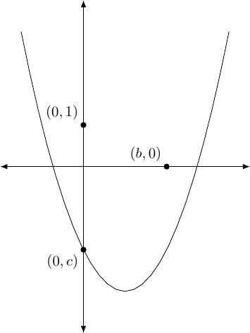
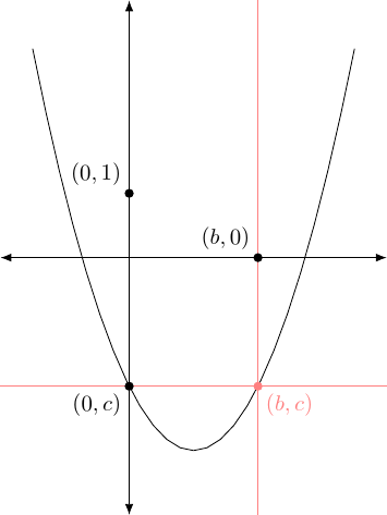
1. Construct the point $(b,c)$ (one method is to construct perpendicular bisectors of the axes at $(b,0)$ and $(0,c)$ and then take the intersection). This is done in Figure 2.

   

   Figure 2: Adding the point $(b,c)$.

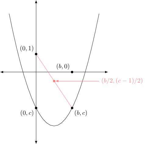
2. Construct the midpoint of $(b,c)$ and $(0,1)$ as in Figure 3.

   

   Figure 3: Adding the midpoint of $(b,c)$ and $(0,1)$.

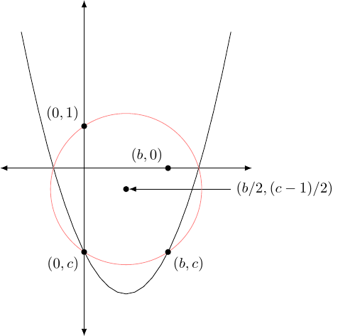
3. Draw the circle with centre at that midpoint which passes through $(b,c)$ (and thus also $(0,1)$), as shown in Figure 4.

   

   Figure 4: The circle with centre at the midpoint of $(b,c)$ and $(0,1)$.

4. The intersections of this circle with the $x$–axis are the solutions of the quadratic (and if there are no intersections then there are no solutions), see Figure 5.

   

   Figure 5: The intersections of this circle with the $x$–axis are the roots.

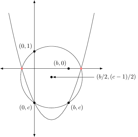
If starting with the more general quadratic $a{x}^2+bx+c$, the initial step is to divide $b$ and $c$ by $a$ and change the sign of $b$. The latter is cosmetic: it is simpler to work with the negative of the $x$–coefficient than the $x$–coefficient itself. The former is because going from an $x^2$–coefficient of $1$ to a coefficient of $a$ is achieved by a scaling in the $y$–direction only and therefore the desired circle becomes an ellipse. As this is not constructible with a ruler and compass, it is necessary to undo this scaling before applying the method.

3 Why it Works

The secret to why it works lies in cyclic quadrilaterals. There are two quadrilaterals that are constructed from the coefficients of the quadratic and its roots (and the point $(0,1)$). These quadrilaterals are cyclic, meaning that the vertices of each lie on a circle called the circumcircle. In fact, the circumcircles are the same and that is the key to finding the roots.

The first quadrilateral is an isosceles trapezium. The four points are the two roots (lying on the $x$–axis) and the points $(0,c)$ and $(-b,c)$. Let us call the roots $\alpha$ and $\beta$. This trapezium is illustrated in Figure 6.

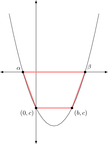
Note that all four points lie on the quadratic curve since $0^2-b\times 0+c=c$ and $b^2-b\times b+c=c$. The roots sum to $b$ so they lie equi-distant from the point $(b/2,0)$. The midpoint of the lower line is $(b/2,c)$. Hence the trapezium is isoscelene, and thus is cyclic. Note that we have used the fact that the sum of the roots is $b$.

To construct the other quadrilateral, we use the fact that the product of the roots is $c$. When working with ruler and compass constructions, multiplication involves constructing similar triangles. So we construct some similar triangles. All of the triangles have $(0,0)$ as one vertex. Then the four triangles have other vertices consequetive pairs from the list $(0,1)$, $(\alpha ,0)$, $(0,c)$, and $(\beta ,0)$ where the list is considered cyclically, as in Figure 7.

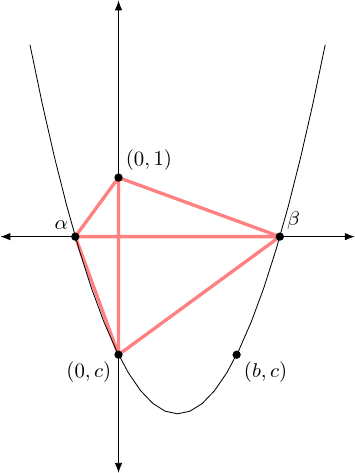
The triangles $\{(0,0),(0,1),(\alpha ,0)\}$ and $\{(0,0),(\beta ,0),(0,c)\}$ are similar since $\alpha \beta =c$. For the same reason the other two triangles are similar. This means that the quadrilateral formed by the outer four vertices has the property that opposite angles add up to $\pi$ and this implies that it is cyclic.

The two cyclic quadrilaterals share three vertices, namely $(0,c)$ and the two roots, and therefore their circumcircles coincide. From the first description, the points $(0,c)$ and $(b,c)$ lie on the circle and so the $x$–coordinate of the centre is $b/2$. From the second description, the points $(0,1)$ and $(0,c)$ lie on the circle and so the $y$–coordinate of the centre is $(c-1)/2$.

Thus the centre has coordinate $(b/2,(c-1)/2)$. As we have assumed that we are given the lengths $b$, $c$, and $1$ we can easily construct this centre. We can also construct a point on its circumference, and thus can construct the circle. By construction, where it intersects the $x$–axis are the roots of the polynomial.

4 Conclusion

That it is possible to solve quadratics with ruler and compass is not a surprise. The quadratic formula involves nothing more involved than addition, multiplication, and square roots, all of which are constructible. What is pleasantly surprising is the simplicity of the method. Indeed, if the axes and the points $(b,c)$ and $(0,1)$ are assumed given at the start then the method involves remarkably few "moves" and might well appeal to the more geometrically minded student who is learning about solving quadratics.