1 Introduction

In this post, I described an activity using quadratics to draw the Batman Logo. It was slightly inspired by the famous Batman Curve, but based on a different version of the Batman logo. One key difference was that my version was presented as a series of quadratics and lines outlining a region, whereas the original Batman Curve was expressed as a single curve.

Slightly out of idle curiosity, I wondered about making my version also into a single curve. I decided to take a different approach to the original Batman Curve, which exploits some features of computer graphics systems, and make much use of the absolute value function.

2 The Absolute Value Function

If functions were superheros, the absolute value function would definitely not be Batman. It would have to be one that had a secret identity as someone very unassuming, and Bruce Wayne is just too flamboyant. On the other side, the superhero part would have to be very powerful indeed. So we're talking someone like Clark Kent, Peter Parker, or Carol Danvers here.

The absolute value function is formally defined as:

$$\mid x\mid =\{\begin{array}{ll}x& x\ge 0\\ -x& x<0\end{array}$$

Less formally, it forces what is inside it to be positive. So $\mid -3\mid =3$. In computing, it is one of the simplest functions to implement as it just throws away the sign of the number.

And yet it can do so much. What we need to use it for is to define the maximum and minimum of two things.

$$\begin{array}{rl}\max (a,b)& =\frac{1}{2}(a+b+\mid a-b\mid )\\ \min (a,b)& =\frac{1}{2}(a+b-\mid a-b\mid )\\ \end{array}$$

We can also feed in functions into these and they give the pointwise maximum and minimum of those functions, as in Figure 1.

I want to use a more compact notation for these, particularly when functions are concerned:

$$\begin{array}{rl}f\wedge g& =\min (f,g)\\ f\vee g& =\max (f,g)\end{array}$$

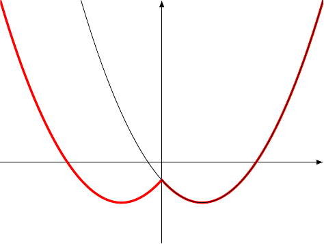
There is another use of the absolute value function. Given a function, say $f(x)$, we can consider $f(\mid x\mid )$. This has the effect of taking the part of the function on the positive $x$–side and reflecting it onto the negative $x$–side as in Figure 2.

3 Batman in Quadratics

Although the absolute value is not Batman, we'll stick to the Batman Logo1. I don't know of another logo that is so distinctive, but also relatively straightforward to draw.

I'm going to modify it slightly, though, as when I drew up the original I was more concerned with the numbers in the coefficients than any other feature. It'll be useful to have the upper and lower parts of the curve meet at "nice" coordinates. Also, the original was upside-down to delay the reveal but for this I'll turn it back the right way. The starting functions are therefore:

1. $y=-0.1x^2+14.1$

2. $y=0.05x^2+4$

3. $y=-0.25x^2+4.5x-16.15$

4. $y=-0.25x^2-4.5x-16.15$

5. $y=-0.3x^2+2.7x-5$

6. $y=-0.3x^2-2.7x-5$

7. $y=10x+14$

8. $y=-10x+14$

9. $y=5x+3$

10. $y=-5x+3$

11. $y=5.5$

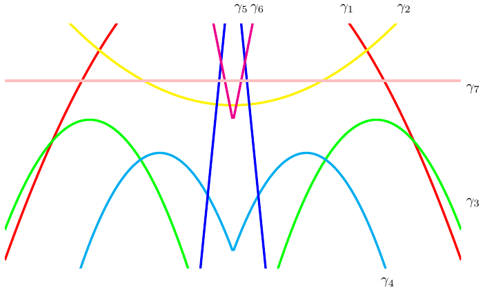
Several of these are in pairs, where one is a reflection of the other in the $y$–axis. We can use the "inner absolute value" trick to condense these into a single function. This leaves us with the following list, illustrated in Figure 3:

1. ${\gamma }_1:y=-0.1x^2+14.1$

2. ${\gamma }_2:y=0.05x^2+4$

3. ${\gamma }_3:y=-0.25x^2+4.4\mid x\mid -16.15$

4. ${\gamma }_4:y=-0.3x^2+2.7\mid x\mid -5$

5. ${\gamma }_5:y=-10\mid x\mid +14$

6. ${\gamma }_6:y=5\mid x\mid +3$

7. ${\gamma }_7:y=5.5$

4 Maxing Out

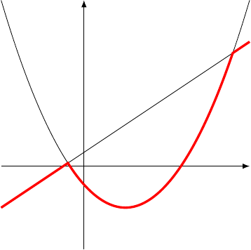
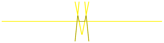
The lower part of the logo is the simplest. This is defined by curves ${\gamma }_3$ and ${\gamma }_4$ and we simply take their maximum, as in Figure 4. Thus:

$${\gamma }_{low}={\gamma }_3\vee {\gamma }_4$$

The upper part would be as simple if it were not for the head. That takes a little more thought. The inner part is the maximum of the lines ${\gamma }_6$ and ${\gamma }_7$, after which we take the minimum of that with ${\gamma }_5$, as in Figure 5. Thus:

$${\gamma }_{head}={\gamma }_5\wedge ({\gamma }_6\vee {\gamma }_7)$$

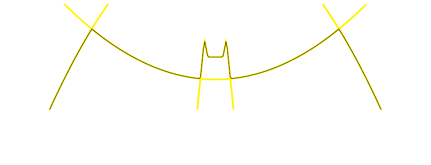
The inner part of the upper curve is then the maximum of this and ${\gamma }_2$, and the full upper curve is the minimum of that with ${\gamma }_1$ as in Figure 6:

$${\gamma }_{high}={\gamma }_1\wedge ({\gamma }_2\vee ({\gamma }_5\wedge ({\gamma }_6\vee {\gamma }_7)\left)\right)$$

5 Tracing the Bat

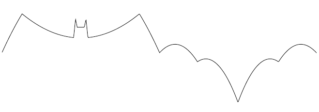
We now have the upper and lower parts of the logo expressed as the graphs of functions. To put them together, though, requires treating them as parametrised curves. Thus rather than plotting $y={\gamma }_{low}(x)$, we have to plot $(x(t),y(t))=(t,{\gamma }_{low}(t))$. This is because the graph of a function cannot double back on itself horizontally. So what we want to do is something like:

$$t\mapsto \{\begin{array}{ll}(t,{\gamma }_{low}(t))& -11\le t\le 11\\ (22-t,{\gamma }_{high}(22-t))& 11\le t\le 33\end{array}$$

Only we'd like to do it without calling on a piecewise definition. Note that our adjustments to the functions mean that the upper and lower curves intersect at $x=\pm 11$.

What we will do to achieve this is the following2. We start by creating a function that first traces out the upper path and then the lower (due to the nature of our functions, we can create that quite simply). This function will form the $y$–coordinate of our path. The "backtracking" will result from what happens to the $x$–coordinate. While the $y$–coordinate is along the upper part of the curve, the $x$–coordinate should simply increase, then when the $y$–coordinate moves to the lower part, the $x$–coordinate should reverse.

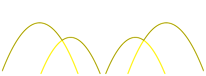
To form the $y$–coordinate path, we start by translating the upper and lower paths so that they are side-by-side3 as in Figure 7.

$${\gamma }_y(t)={\gamma }_{high}(t+11)\vee {\gamma }_{low}(t-11)$$

The $x$–coordinate path just needs to go from $-11$ to $11$ and back again.

$$\begin{array}{rl}{\gamma }_x(t)& =11-\mid t\mid \\ {\gamma }_y(t)& ={\gamma }_{high}(t+11)\vee {\gamma }_{low}(t-11)\end{array}$$

1

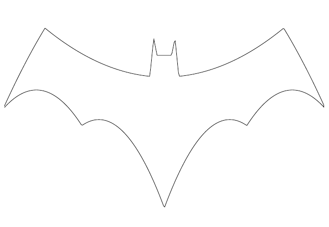
Putting that together, we get our final curve as:

$$\beta (t)=({\gamma }_x(t),{\gamma }_y(t))$$

6 Unrolling the Curves

Mathematical notation is designed to focus attention. By hiding unnecessary details, it allows us to work on what is important or relevant without getting lost in a morass of symbols. The form of our curve in Equation 1 has this property. We can see enough of the definition without having to know too much about how ${\gamma }_{low}$ and ${\gamma }_{high}$ are defined.

It is with some trepidation, therefore, that I am going to unroll the definition of ${\gamma }_y$ back to a function of $t$.

Thanks to the left and right shifts, we can rearrange the final form of ${\gamma }_y$ slightly.

$$\begin{array}{rl}{\gamma }_y(t)& ={\gamma }_{high}(t+11)\vee {\gamma }_{low}(t-11)\\ & =({\gamma }_1(t+11)\vee {\gamma }_3(t-11)\vee {\gamma }_4(t-11))\\ & \phantom{=}\wedge ({\gamma }_2(t+11)\vee ({\gamma }_5(t+11)\wedge ({\gamma }_6(t+11)\vee {\gamma }_7(t+11))\left)\right)\\ & =((-0.1t^2-2.2t+2)\vee (-0.25t^2+5.5t-46.4+4.4\mid t-11\mid )\\ & \phantom{=(}\vee (-0.3t^2+6.6t-41.3+2.7\mid t-11\mid ))\\ & \phantom{=}\wedge ((0.05t^2+1.1t+10.05)\vee ((-10\mid t+11\mid +14)\wedge ((5\mid t+11\mid +3)\vee 5.5)\left)\right)\\ & =\begin{array}{ccc}\left(\begin{array}{c}-0.1t^2-2.2t+2\\ \vee \\ -0.25t^2+5.5t-46.4+4.4\mid t-11\mid \\ \vee \\ -0.3t^2+6.6t-41.3+2.7\mid t-11\mid \end{array}\right)& \wedge & \left(\begin{array}{c}0.05t^2+1.1t+10.05\\ \vee \\ \left(\begin{array}{c}-10\mid t+11\mid +14\\ \wedge \\ \left(\begin{array}{c}5\mid t+11\mid +3\\ \vee \\ 5.5\end{array}\right)\end{array}\right)\end{array}\right)\end{array}\end{array}$$

Putting the $x$ and $y$ parts together, we get:

$$\left(\begin{array}{c}11-\mid t\mid ,\begin{array}{ccc}\left(\begin{array}{c}-0.1t^2-2.2t+2\\ \vee \\ -0.25t^2+5.5t-46.4+4.4\mid t-11\mid \\ \vee \\ -0.3t^2+6.6t-41.3+2.7\mid t-11\mid \end{array}\right)& \wedge & \left(\begin{array}{c}0.05t^2+1.1t+10.05\\ \vee \\ \left(\begin{array}{c}-10\mid t+11\mid +14\\ \wedge \\ \left(\begin{array}{c}5\mid t+11\mid +3\\ \vee \\ 5.5\end{array}\right)\end{array}\right)\end{array}\right)\end{array}\end{array}\right)$$