Intermediate Axes
2019-04-02

1 Introduction
This is a follow-up to a post on The Aperiodical about a Many-to-many Shape Sorter. The post is about designing solids which look like different shapes from different angles. After reading it, I came up with a solid that looked like a circle, a square, and a hexagon when viewed along each of the principle axes.
A key part of figuring out the solid was looking at the diameters of a (2D) shape and realising that any sufficiently reasonable shape will have two orthogonal diameters of the same length. In explaining my design in a comment on the original post, I remarked that this was a consequence of the Intermediate Value Theorem. In the interests of completeness, this is a write-up of that statement.
2 Diameters
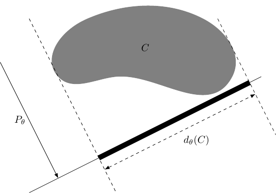
We first need to define what we mean, in this article, by the diameter of a shape in the plane. We do not mean the distance between two points in the shape, but rather the length of its "shadow" when projected onto a line.
Let be a bounded connected subset. For , let be the line through the origin at angle to the –axis. Let be the orthogonal projection onto .
The diameter of at angle is the length of the interval .
We shall write this diameter as .
The result that we want to show is that a "reasonable" shape has two orthogonal diameters that are the same. We focus on the boundary of the shape as the shadow cast by a bounded shape is the same as that cast by its boundary.
Let be a simple, closed curve in with a continuous parametrisation. Then there is such that:
3 Proof
The proof is similar to that of "stabilising a wobbly table". The idea is to consider pairs of diameters for orthogonal angles. As we rotate the shape, these diameters vary continuously. After rotating the shape by a right-angle, the original diameters are swapped. This means that there must have been a rotation where the two diameters were the same.
The key is to show that the diameter varies continuously.
Let be a simple, closed curve with a continuous parametrisation. Then the function is continuous.
Let be a parametrisation of . As the shape is closed, we have .
For , the projection map is defined by:
This is clearly continuous in . Thus is the image of the continuous function:
The domain of this function is . It therefore lives in the space of continuous functions . The key property of this space that we want to use is that there is an isomorphism:
Namely, the function:
is continuous as a map from to .
This is a standard result in functional analysis (with overtones of category theory). For completeness, we shall prove it at the end.
The functions and are continuous on almost by definition:
and similarly for the minimum.
This means that the following compositions are continuous:
whence, finally, the following map is continuous:
This is precisely , and so this function is continuous as required.
Now the function actually has period . Therefore the continuous function:
has the property that:
At this juncture, the Intermediate Value Theorem steps in to show that there is some such that . That is to say, that:
and hence that has two orthogonal diameters of the same length.
4 The Technical Details
The technical result that we needed was that there is a homeomorphism:
This is a special case of a standard result which can be phrased in terms of enriched category theory and states that:
In the category of topological spaces enriched over itself, compact Hausdorff spaces are exponential objects.
(See the nlab for more.)
This is the sort of result whereby if you understand what all of those words mean, you are probably already sufficiently familiar with it that you don't need to see a proof here. We will therefore prove just the result we need in more elementary language.
There is a natural homeomorphism:
The map is defined in the obvious manner: given we define by . The inverse is: given , define by .
Assuming that these are well-defined, they are clearly inverse to each other.
We then need to prove the following:
-
For , is continuous.
-
The map is continuous.
-
The maps and are continuous. Once it is established that they are well-defined, it is enough to establish that, say, is an isometry.
As everything in sight is a metric space, we will use the characterisation of continuity as that of taking convergent sequences to convergent sequences.
-
Fix and . Let be a convergent sequence in .
Then the sequence is convergent in with limit . As is continuous, .
Then and so . Hence takes convergent sequences to convergent sequences, whence is continuous.
-
Fix . Let be a convergent sequence in .
Write and . Then and .
Now . Since , and is continuous, . Convergence in is uniform convergence, and therefore we have that:
Therefore as and we have that . Hence is continuous.
-
To show that is an isometry, we just need to consider the definitions of the norms on each side.
Hence is an isometry and so as it has an inverse it is an isomorphism.