1 Introduction

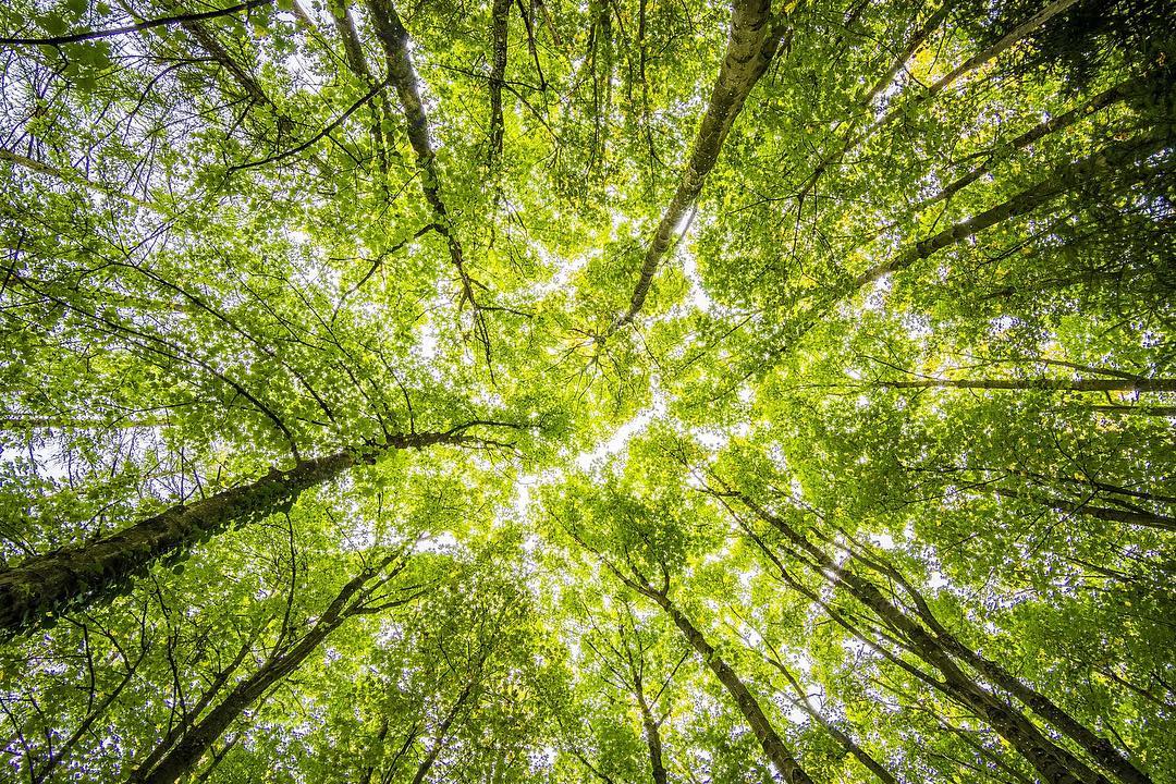
I recently saw the picture, Figure 1, of a forest canopy taken from the ground1. The light through the leaves showed definite lines where the leaves from one tree met the leaves from another. The original context in which I saw the image was about how relaxing it would be to be in the forest, looking up at the canopy.

My reaction on seeing it was to think of Voronoi Diagrams.

2 Voronoi Diagrams

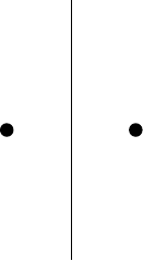
Voronoi diagrams are fairly simple to understand. Start with a set of points on the plane (or piece of paper) and then divide the plane (or paper) into regions based on which point is closest.

With just two points, the dividing line is the perpendicular bisector between them, as in Figure 2.

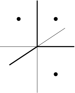
With more than two points, a naive method2 of drawing the boundaries of the regions is to draw all the bisectors between the points and then figure out which parts define the regions.

Another method, which is quite fun to watch, is to fill ever increasing circles centred at each point but to never fill in a place that's already been filled.

Anyway, back to the trees. Inspired by the picture, I wondered if anyone had used Voronoi diagrams to study tree canopies. It turned out that they had (many thanks to the people on twitter who pointed me in this direction). The phenomenon whereby the boundaries are visible is called canopy shyness and some papers have been written using Voronoi diagrams as a tool to study this.

3 Generalised Voronoi Diagrams

Full confession: I've not yet read the papers. I need to set aside time to read them, particularly as I suspect they won't be aimed at me (a Mathematician) so I'll have a bit of translation to do when reading them. Nevertheless, it's still an interesting topic and, as usual, it sparked me off on a little mathematical journey of my own which, in all likelihood, has no particular relevance to tree growth but which is nevertheless inspired by it.

One thing that particularly struck me about the original image was how well-defined and above all straight the gaps were. On the face of it, this seems reasonable: the branches from each tree grow outward until they get near to a space already occupied by the branches from another tree. This is exactly the situation that Voronoi diagrams describe.

But that assumes two things: that the trees all grow at the same speed and that they started at the same time.

What if we relax those conditions?

3.1 General Voronoi Diagrams

Before looking at what happens if the trees grow at different speeds and at different times, let's examine the general case to establish some notation.

We suppose that we have some points in the plane, say $\left\{a_i\right\}$, and each is a source of growth. We additionally assume that the growth is defined by a radial function, say $r_i(t)$, in that the unfettered growth from $a_i$ at time $t$ is a circle of radius $r_i(t)$.

Each function $r_i(t)$ has the structure that there is some time $t_i$ such that $r_i(t)$ is zero for $t<t_i$, and for $t>t_i$ then it is strictly increasing. This means that once the growth starts, the function from time to radius is invertible – i.e., knowing the radius we can (in theory) figure out the time it got there.

By "unfettered growth" I mean that the growth if no obstruction were present.

For a point $x$, to figure out which source gets to $x$ we need to look at the distances from $x$ to each point $a_i$. This is done using the Euclidean distance function, written $\parallel x-a_i{\parallel }_2$, which is none other than Pythagoras' theorem in disguise. For each point, we can then work out the time at which $r_i(t)=\parallel x-a_i{\parallel }_2$ which would be the time when the growth from $a_i$ would reach $x$. The earliest time "wins".

Since we've assumed that $r_i(t)$ is invertible (at least for $t>t_i$), these times are given by:

$$t_{x,i}=r_i^{-1}(\parallel x-a_i{\parallel }_2)$$

To find the boundary between two regions, we need to figure out those points $x$ which are reached from two source points, say $a_1$ and $a_2$, at the same time. This means that we need to find $x$ such that $t_{x,1}=t_{x,2}$, which means solving:

$$r_1^{-1}(\parallel x-a_1{\parallel }_2)=r_2^{-1}(\parallel x-a_2{\parallel }_2)$$

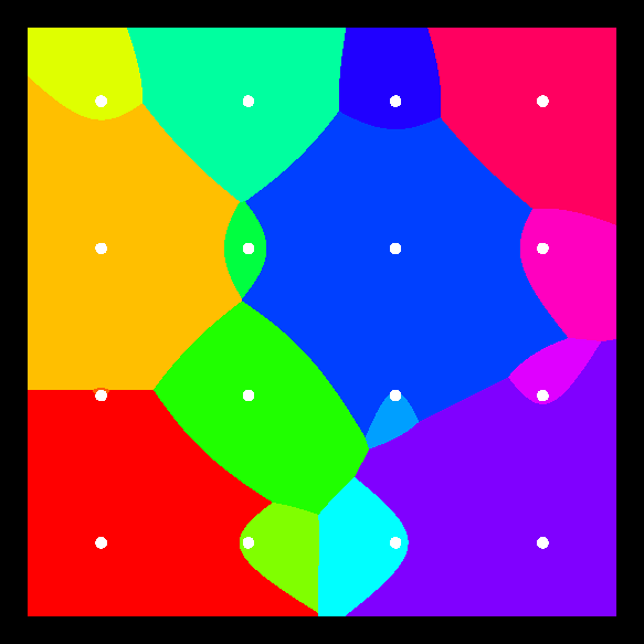
In the next sections I'll look at this equation for particular circumstances. As those circumstances get more complicated, I'll be able to say less in general. To counteract that, here's a Voronoi playground. It places a number of points in a square and generates the Voronoi diagram. You can move the points around. You can choose one of the types of Voronoi diagram referred to below, if there are any parameters then it generates them randomly within a reasonable range.

3.2 Weighted Voronoi Diagrams

The easiest one to work with is if the trees grow at different speeds. Each tree, located at point $a_i$, has a speed, say $s_i$, such that its unfettered growth function is given by:

$$r_i(t)=\{\begin{array}{ll}0& t\le 0\\ s_{i}t& t>0\end{array}$$

Thus the boundaries between two regions are those $x$ for which:

$$\frac{1}{s_i}\parallel x-a_i{\parallel }_2=\frac{1}{s_j}\parallel x-a_j{\parallel }_2$$

Rearranging this, say for $a_1$ and $a_2$, produces an equation of the form:

$$\parallel x-a_1{\parallel }_2=k\parallel x-a_2{\parallel }_2$$

where $k$ is some (positive) constant. This is a circle.

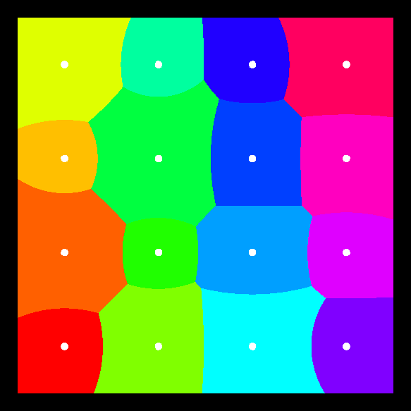
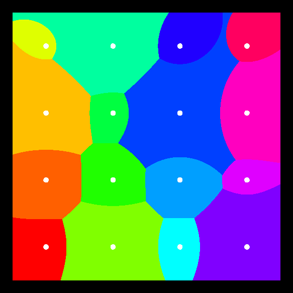
Such Voronoi diagrams are called weighted Voronoi diagrams. The boundaries are made up from arcs of circles, as in Figure 4.

3.3 Shifted Voronoi Diagrams

The second possible change would be to have the trees start growing at different times, say at time $t_i$ from point $a_i$, but at the same speed. The unfettered growth function would then be of the form

$$r_i(t)=\{\begin{array}{ll}0& t\le t_i\\ t-t_i& t>t_i\end{array}$$

Thus the boundaries between two regions is given by finding $x$ such that:

$$\parallel x-a_i{\parallel }_2+t_i=\parallel x-a_j{\parallel }_2+t_j$$

This rearranges to an equation of the form, for $a_1$ and $a_2$:

$$\parallel x-a_1{\parallel }_2=\parallel x-a_2{\parallel }_2+k$$

where $k$ can be any real number3.

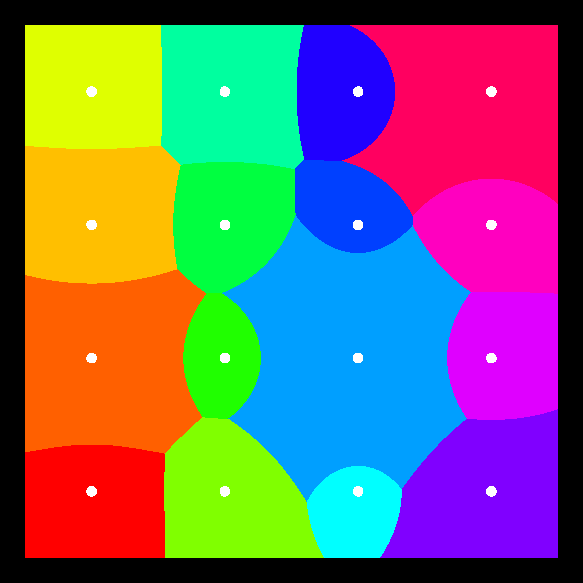
This is the focus-focus property of a hyperbola4. Thus in this case the boundaries of the Voronoi regions will be segments of hyperbolae, as in Figure 5.

3.4 Shifted, Weighted Voronoi Diagrams

We're doing quite well with conic sections here, but sadly all good things come to an end. If we allow both shifting and weighting then we get equations of degree $4$.

Our unfettered growth functions now look like:

$$r_i(t)=\{\begin{array}{ll}0& t\le t_i\\ s_i(t-t_i)& t>t_i\end{array}$$

and this means that we are solving equations of the form:

$$\frac{1}{s_i}\parallel x-a_i{\parallel }_2+t_i=\frac{1}{s_j}\parallel x-a_j{\parallel }_2+t_j$$

which rearranges to something of the form:

$$\parallel x-a_1{\parallel }_2=k\parallel x-a_2{\parallel }_2+c$$

To see what this looks like, let us transform the points so that $a_1$ and $a_2$ lie on the $x$–axis, say at $(-1,0)$ and $(1,0)$.

Our equation is thus:

$$\parallel (x,y)-(-1,0){\parallel }_2=k\parallel (x,y)-(1,0){\parallel }_2+c$$

Squaring both sides, we can replace the $\parallel \cdot {\parallel }_2$ by the Pythagorean identity:

$$(x+1{)}^2+y^2=k^2(x-1{)}^2+k^2{y}^2+2kc\parallel (x,y)-(1,0){\parallel }_2+c^2$$

Expanding out the brackets and gathering terms, we get:

$$(1-k^2)x^2+2(k^2+1)x+(1-k^2)y^2+(1+k^2+c^2)=2kc\parallel (x,y)-(1,0){\parallel }_2$$

To see the "wood for the trees5", let's hide some of the mess and write this as:

$${\alpha }_1{x}^2+{\alpha }_{2}x+{\alpha }_3{y}^2+{\alpha }_4={\alpha }_5\parallel (x,y)-(1,0){\parallel }_2$$

The $\parallel \cdot {\parallel }_2$ part is secretly a square root, so we square both sides again to get:

$$\begin{array}{rl}{\alpha }_1^2{x}^4& +{\alpha }_2^2{x}^2+{\alpha }_3^2{y}^4+{\alpha }_4^2\\ & +2({\alpha }_1{\alpha }_2{x}^3+{\alpha }_1{\alpha }_3{x}^2{y}^2+{\alpha }_1{\alpha }_4{x}^2+{\alpha }_2{\alpha }_{3}x{y}^2+{\alpha }_2{\alpha }_{4}x+{\alpha }_3{\alpha }_4{y}^2)\\ & ={\alpha }_5^2((x-1{)}^2+y^2)={\alpha }_5^2{x}^2-2{\alpha }_5^{2}x+{\alpha }_5^2+{\alpha }_5^2{y}^2\end{array}$$

Gathering everything together, and relabelling again, the general form is:

$$p_{4,0}{x}^4+p_{3,0}{x}^3+p_{2,0}{x}^2+p_{1,0}x+p_{0,4}{y}^4+p_{0,2}{y}^2+p_{2,2}{x}^2{y}^2+p_{1,2}x{y}^2+p_{0,0}=0$$

which is a quartic. This means that the boundaries of the regions in the Voronoi diagram could be quite complicated, as in Figure 6.

3.5 Ever Decreasing Circles

Back to thinking about trees, I do think that the unfettered growth model has its flaws. A tree with no competitors would not spread out indefinitely. Most likely, there would be some maximum spread and that as it reached that distance, the growth would gradually slow. A possibly model for this would be:

$$r_i(t)=\{\begin{array}{ll}0& t\le t_i\\ M_i(1-e^{-k_i(t-t_i)})\end{array}$$

The inverse of this function (for $t>t_i$) is given by:

$$r_i^{-1}(x)=-\frac{1}{k_i}\log (1-\frac{x}{M_i})+t_i$$

This isn't actually as scary as it looks. In particular, if all the $M_i$ are the same, say $M$, then this is of the form:

$$r_i^{-1}(x)=\frac{1}{k_i}g(x)+t_i$$

where $g(x)=-\log (1-\frac{x}{M})$. This looks like the shifted, weighted Voronoi diagram but with a different notion of what distance is, as in Figure 7.

4 As the Duck Waddles or as the Tree Grows

I'll end with a comment on where I can see a limitation of Voronoi diagrams as I've described them above. It is entirely possible that this is known about, and dealt with, in the literature but as that's still on my "to read" list then I don't know.

Let's go back to the weighted Voronoi diagram and consider the situation with two points. The Voronoi diagram looks a little like Figure 8.

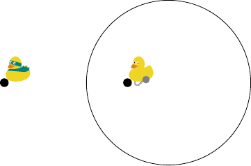
Now the diagram shows the plane divided into two regions. These two regions are defined by which duck would reach a point first (clearly the superhero duck would be faster than the duck with the ball and chain).

But here's the thing: to get to some of those points first, the superhero duck would have to fly through the region that the prison duck controls. That is, the criteria for "getting there first" is by the most direct route.

With trees, that route might not be available. If the slower growing tree has filled a region then the faster one won't send branches through it to reach the other side, it will have to go around. So the actual shape won't be a circle, but will extend somewhat to (in this case) the right-hand side. Possibly more of the shape in Figure 9.

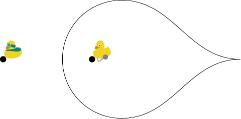
In this case, the metric used to measure the distance between two points will be the path metric which measures it by the length of the shortest path. Normally this agrees with the Euclidean metric, but when there are excluded regions then it can be more complicated.

Something to investigate!