1 Introduction

Triangles have been acknowledged as the atoms of shapes for many a year. In Euclidiastes, we find such exhortations as:

"Triangles! Triangles! All is triangles!" says the mathematician.

This pervades literature even to the modern times, as we find in The Geometer who Computed by Herself:

"But still I am the geometer who computes by herself, and all triangles are alike to me."

With such a history, it is unsurprising that present day exponents of the art of computer graphics should turn to triangles when drawing complex shapes on the screen. However, while the Geometer who Computed by Herself would claim that all triangles are alike, sometimes a triangle needs to know that it is part of a larger whole to truly know how to behave.

The simplest shape that a triangle can be a true part of is a quadrilateral, since a quadrilaterals can be built up from two triangles sharing a common side. The claim is, then, that there is a difference between a quadrilateral composed of two triangles, and two triangles that happen to share a common side.

2 Filling in the Evidence

Consider the two quadrilaterals in Figure 1: a parallelogram and a trapezium. Both are composed of two triangles (with the dividing line going from bottom left to top right). The aim is to shade each from left to right, with colour from white to black. This is done by specifying a colour for each vertex of each triangle and interpolating the colour in between. The point here is that each (internal) point of a triangle has a unique expression of the form:

$$\stackrel{\rightharpoonup }{v}=\alpha \stackrel{\rightharpoonup }{a}+\beta \stackrel{\rightharpoonup }{b}+\gamma \stackrel{\rightharpoonup }{c}$$

where $\stackrel{\rightharpoonup }{a},\stackrel{\rightharpoonup }{b},\stackrel{\rightharpoonup }{c}$ are the vertices of the triangle and $\alpha ,\beta ,\gamma$ are real numbers satisfying $\alpha +\beta +\gamma =1$. The numbers $\alpha$, $\beta$, and $\gamma$ can then be used to interpolate any quantity from the corners into the triangle. In particular, if the corners are assigned colours, say $C_a$, $C_b$, and $C_c$, then the point $\stackrel{\rightharpoonup }{v}$ is given the colour

$$\alpha C_a+\beta C_b+\gamma C_c.$$

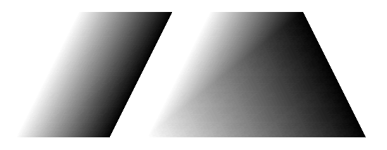
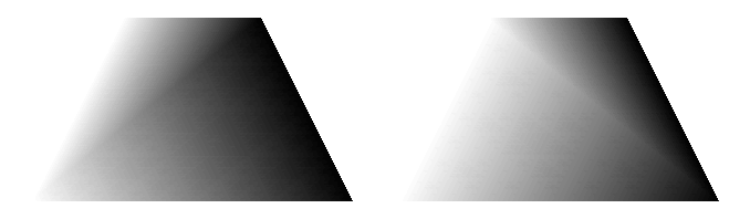
As can be seen, this works well for the parallelogram but not well for the trapezium. There is a distinct line from bottom left to top right showing how the trapezium has been divided into triangles. Indeed, if we split it the other way then we get a different colouring, as in Figure 2.

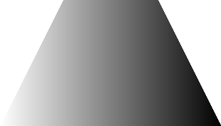
For the trapezium, a possible solution is to shade it strictly from left to right as in Figure 3. However, then the sides are not uniformly coloured but are themselves shaded. This is not ideal, particularly if the trapezium is itself part of a larger picture, and gets less usable if the quadrilateral is more irregular.

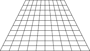
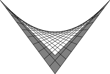
The problem is shown even more clearly if we map a texture, such as a grid, to the quadrilateral as in Figure 4. It is obvious what is happening here. In going from the parallelogram to the trapezium we are distorting one triangle only. The other triangle is left alone.

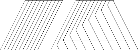
The grid picture also provides the solution. It is obvious what the picture should look like: the lines running from top to bottom to should gradually change from the left hand edge to the right hand edge but should never have bends, as in Figure 5.

3 Pointing to a Solution

There is no linear transformation that will take an ordinary square or rectangle to a trapezium, or more general quadrilateral. Therefore defining coordinates using linear transformations is not possible and we have to allow for more general coordinate systems.

The thing to notice about Figure 5 is that all of the "vertical" lines have a common intersection point. So to find out which line a point lies on, we need to first compute the intersection point and work from there.

We already know two of the lines: the first and last. So we can work out the intersection point from these.

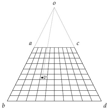
Let's label the vertices of the trapezium as in Figure 6 with $o$ as the intersection point. We also want an arbitrary point inside, say $v$. The whole problem is translation-invariant and so we can assume that one of our points is at the origin. For reasons that will become clear later, we do not want to assume that this is $o$, so we pick one of the vertices. Thus we assume without loss of generality that $a$ is at the origin.

The intersection point, $o$, lies on the lines $a-b$ and $c-d$. It can therefore be written as both $tb$ and $sc+(1-s)d$. That is, we look for $s$ and $t$ such that:

$$tb=sc+(1-s)d$$

1

We actually only need to know one of them. We can remove the other by a judicious dot product. For any vector, say $u$, let us write $\hat{u}$ for the vector obtained by rotating $u$ anticlockwise by $\pi /2$. Then $u\cdot \hat{u}=0$ and $w\cdot \hat{u}=-u\cdot \hat{w}$.

We take dot products of both sides of 1 by $\hat{c}-\hat{d}$ to get:

$$tb\cdot (\hat{c}-\hat{d})=sc\cdot (\hat{c}-\hat{d})+(1-s)d\cdot (\hat{c}-\hat{d})=-sc\cdot \hat{d}+d\cdot \hat{c}-sd\cdot \hat{c}=d\cdot \hat{c}$$

which simplifies to:

$$t=\frac{d\cdot \hat{c}}{b\cdot (\hat{c}-\hat{d})}.$$

2

There is a danger that the denominator could be zero. For this to happen, the two lines $a-b$ and $c-d$ would have to be parallel. For now, we shall merely note that this is a special case and assume that it is not true.

Thus the intersection point is:

$$o=\frac{d\cdot \hat{c}}{b\cdot (\hat{c}-\hat{d})}b.$$

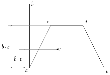
Now we consider the line $o-v$. We want to know how far this is from the line $a-b$ towards $c-d$. To do this, we compute its intersection with the line $a-c$. This intersection point will have the formula $xc$ (since $a$ is at the origin) and the value of $x$ will be the coordinate that we want. Points on the line $o-v$ have the formula $v+r(o-v)$ so we're looking for:

$$v+r(o-v)=xc.$$

As before, we use $\hat{o}-\hat{v}$ to get rid of the $r$ and end up with:

$$v\cdot \hat{o}=xc\cdot (\hat{o}-\hat{v})$$

which rearranges to:

$$x=\frac{v\cdot \hat{o}}{c\cdot (\hat{o}-\hat{v})}=\frac{\hat{v}\cdot o}{\hat{c}\cdot (o-v)}.$$

3

Before we substitute in for $o$, let us note that as this expression is a fraction, we can multiply top and bottom by the same quantity. Since also $o$ involves fractions, this means that we can clear the fractions in $o$. In other words, instead of substituting in the above formula for $o$, we first write:

$$o-v=\frac{d\cdot \hat{c}}{b\cdot (\hat{c}-\hat{d})}(b-\frac{b\cdot (\hat{c}-\hat{d})}{d\cdot \hat{c}}v).$$

We ignore the leading fraction, and take the dot product of this with $\hat{c}$ to get:

$$b\cdot \hat{c}-\frac{b\cdot (\hat{c}-\hat{d})}{d\cdot \hat{c}}v\cdot \hat{c}.$$

The numerator, meanwhile, becomes

$$\hat{v}\cdot b=-\hat{b}\cdot v$$

Hence:

$$x=\frac{\hat{b}\cdot v}{\frac{b\cdot (\hat{c}-\hat{d})}{d\cdot \hat{c}}\hat{c}\cdot v-b\cdot \hat{c}}.$$

4

By exchanging $b$ and $c$, we obtain a formula for the $y$–coordinate. Note that $c\cdot \hat{b}=-b\cdot \hat{c}$.

$$y=\frac{\hat{c}\cdot v}{\frac{c\cdot (\hat{b}-\hat{d})}{d\cdot \hat{b}}\hat{b}\cdot v+b\cdot \hat{c}}.$$

5

4 3D

The two formulae, 4 and 5, assume that we are working in ${ℝ}^2$ with one vertex ($a$) at the origin. Our rectangle could be anywhere in $3$–space. Thus our initial data is four $3$–vectors, assumed to live in an affine plane (i.e., a plane not necessarily through the origin). It is easy enough to translate this plane so that one vertex is at the origin by subtracting that vertex from the other three. Dot products are the same irrespective of the ambient space, so the only other ingredient needed is the rotation.

To rotate a vector in a plane, we first find the normal vector to that plane. We can do this using the cross product. This normal vector then defines a rotation of $\pi /2$ by taking the cross product with it. If we note that every term in 4 and 5 involves exactly two rotated vectors, we don't have to normalise the normal vector since all the lengths will cancel.

Thus the algorithm is as follows:

1. Our input is four $3$–vectors, say $a$, $b$, $c$, $d$. We assume that $a$ and $d$ are opposite, as are $b$ and $c$.

2. We make the replacements $b\mapsto b-a$, $c\mapsto c-a$, and $d\mapsto d-a$.

3. We compute the normal vector $n≔b\times c$ and use this to compute $\hat{b}≔n\times b$, $\hat{c}≔n\times c$, and $\hat{d}≔n\times d$.

4. We store the numbers $b\cdot \hat{c}$, $\frac{c\cdot (\hat{b}-\hat{d})}{d\cdot \hat{b}}$, and $\frac{b\cdot (\hat{c}-\hat{d})}{d\cdot \hat{c}}$ and the vectors $a$, $\hat{b}$, and $\hat{c}$ (these only need to be computed once for the quadrilateral).

5. For each point $v$ inside the quadrilateral, we replace $v$ by $v-a$ and compute $x$ and $y$ according to 4 and 5. Note that the quantities where $v$ appears, namely $\hat{b}\cdot (v-a)$ and $\hat{c}\cdot (v-a)$, can be computed for the vertices and interpolated into the interior of the triangles comprising the quadrilateral by the usual barycentric interpolation.

5 Life on the Edge

We should worry about edge cases. The formulae in 4 and 5 involve fractions and so there is a possibility of the denominators being zero. In addition, the reasoning that led to those formulae depended itself on a certain fraction and we should check what happens if that fraction has zero denominator.

Let's start with this latter case. This is where the denominator in 2 is zero. As stated in the following paragraph, this means that the lines $a-b$ and $c-d$ are parallel meaning that the intersection point is "at infinity". In this case, the formula for the $x$–coordinate becomes

$$x=\frac{\hat{b}\cdot v}{-b\cdot \hat{c}}=\frac{\hat{b}\cdot v}{\hat{b}\cdot c}.$$

What this formula is doing is projecting both $v$ and $c$ orthogonally onto the line orthogonal to $b$ and measuring the ratio of the image of $v$ to the image of $c$. More geometrically, this draws lines parallel to $b$ through $v$ and $c$ and finds their intersection points with the line orthogonal to $b$, then measures the height of the point corresponding $v$ relative to that corresponding to $c$. This is exactly what the $x$–coordinate should be in this situation.

The next term to worry about in 4 is the fraction $\frac{b\cdot (\hat{c}-\hat{d})}{d\cdot \hat{c}}$. The denominator of this, $d\cdot \hat{c}$, is zero if $d$ and $c$ are parallel. This means that the quadrilateral is degenerate and is actually a triangle (possibly itself further degenerate) as in Figure 8.

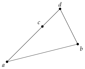
The solution here is straightforward: cycle the vertices round so that the base vertex (viewed as the origin) is opposite the degenerate vertex. Note also that with $c$ as the degenerate vertex, with the triangulation scheme $a-c-d,a-b-d$ then the triangle $a-c-d$ is not rendered. Rotating the labels means that the quadrilateral is divided more equitably between the two triangles.

The decision as to whether to permute the vertices can be taken at the outset, and should be based on the relative sizes of the angles at the vertices. To avoid the situation above, the best vertex to choose as the origin is the one opposite the largest internal angle.

The last danger is with the full denominator in 4. As we have already considered the quantities $d\cdot \hat{c}$ and $b\cdot (\hat{c}-\hat{d})$, we can assume that these are non-zero and thus that the denominator in 4 is a multiple of $\hat{c}\cdot (o-v)$. If this is zero, $c$ and $o-v$ are parallel.

Let us restrict our attention to the case of a convex quadrilateral. Then while our quadrilateral may not be as regular as the trapezium of Figure 6, it nevertheless shares some basic properties with it. In particular, it is contained within the cone emanating from $o$ and bounded by the lines $o-a$ and $o-c$. In particular, every point in the quadrilateral has the form:

$$(1-\lambda )o+\lambda u$$

for some $u$ in the line segment $a-c$ and $\lambda \ge 0$. Then $u$ has the formula $\alpha c$ (since $a$ is the origin) with $\alpha \in [0,1]$. In particular, there is some $\lambda \ge 0$ and $\alpha \in [0,1]$ such that

$$v=(1-\lambda )o+\lambda \alpha c.$$

Rearranging, $v-o=\lambda \alpha c-\lambda o$. Now if we assume that $v-o$ is parallel to $c$, we find that either $v=o$ or $o$ is itself a multiple of $c$.

In the first case, the intersection of $a-b$ and $c-d$ is inside the quadrilateral and hence (by convexity) we must have either $a=c$ or $b=d$ and the quadrilateral is degenerate. In the second case, the points $o-a-c$ are collinear, but so are $o-a-b$ and $o-c-d$ and this means that the quadrilateral in fact collapses to a line.

In conclusion, for convex quadrilaterals then the danger cases all correspond to degenerate cases which can either be dropped altogether (as they won't render) or a simple modification of the initial data removes the degeneracy. To accomplish this, we add a step to the algorithm between the first and second which decides on the best vertex to choose as the anchor.

6 Go Fly a Kite

The above concentrates on convex quadrilaterals. It is possible to consider non-convex quadrilaterals such as darts. However, the correct grid would pass out of the shape and therefore would not be fully renderable. As pleasing as the ideal shape is, as in Figure 9, the fact that only the part in the dart would render means that it would not look like this on a screen.

Thus although the formulae still produce something for non-convex quadrilaterals, they really only make sense when they are convex.

7 Examining the Edges

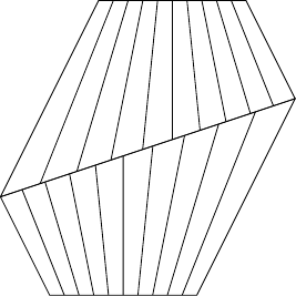
The algorithm above was constructed to fix the issue of interpolation when triangles are part of a larger quadrilateral. Unfortunately, as a correspondent pointed out to me, it itself suffers a similar failing when the quadrilaterals are themselves part of a larger shape. The problem is shown in Figure 10 where the lines do not match (for simplicity, only the "vertical" lines are shown).

It does, though, have linear interpolation along two sides: the two adjacent to the "chosen" vertex (i.e., the one we translate to the origin). This is because the, say, $x$–coordinate is determined by intersecting the line $o-v$ with the line $a-c$ and looking at the ratio of the intersect to the whole segment. If instead we intersected the line $o-v$ with the line $b-d$ we would force linear interpolation on the opposite face.

A balanced approach is to interpolate between these two $x$–values as we sweep from the line $a-c$ to the line $b-d$. To achieve this, we need a parameter that varies from $0$ on the line $a-c$ to $1$ on the line $b-d$. The ideal such parameter would be the angle subtended at the intersection of the lines $a-b$ and $c-d$. However, computing this parameter involves an inverse trigonometric function and thus is more expensive than warranted. A cheaper parameter to use is the computed $y$–coordinate. As we've introduced two $x$–coordinates (corresponding to the lines $a-c$ and $b-d$), we similarly have two $y$–coordinates. Again, we could look for a "best" $y$–coordinate or a cheap one. Probably the cheapest non-biased one is to take the average of the two computed $y$–coordinates.

Equations 4 and 5 now become the computations of $x_0$ and $y_0$. We need similar formulae to compute the values of $x_1$ and $y_1$ at the opposite edges.

Repeating the argument that led to Equation 4, we see that we're looking for the point on the line $v+r(o-v)$ which is also on the line $b+x_1(d-b)$. That is:

$$v+r(o-v)=b+x_1(d-b).$$

We use the same argument as before. We observe that:

$$o-v=\frac{d\cdot \hat{c}}{b\cdot (\hat{c}-\hat{d})}(b-\frac{b\cdot (\hat{c}-\hat{d})}{d\cdot \hat{c}}v),$$

and so taking dot products with $\hat{b}-\frac{b\cdot (\hat{c}-\hat{d})}{d\cdot \hat{c}}\hat{v}$ kills the $r(o-v)$ term to leave:

$$v\cdot (\hat{b}-\frac{b\cdot (\hat{c}-\hat{d})}{d\cdot \hat{c}}\hat{v})=b\cdot (\hat{b}-\frac{b\cdot (\hat{c}-\hat{d})}{d\cdot \hat{c}}\hat{v})+x_1(d-b)\cdot (\hat{b}-\frac{b\cdot (\hat{c}-\hat{d})}{d\cdot \hat{c}}\hat{v}).$$

Removing the obvious zeros, we are left with:

$$v\cdot \hat{b}=-\frac{b\cdot (\hat{c}-\hat{d})}{d\cdot \hat{c}}b\cdot \hat{v}+x_1(d\cdot \hat{b}-\frac{b\cdot (\hat{c}-\hat{d})}{d\cdot \hat{c}}(d-b)\cdot \hat{v})$$

which rearranges to:

$$x_1=\frac{(1-\frac{b\cdot (\hat{c}-\hat{d})}{d\cdot \hat{c}})v\cdot \hat{b}}{d\cdot \hat{b}-\frac{b\cdot (\hat{c}-\hat{d})}{d\cdot \hat{c}}(d-b)\cdot \hat{v}}=\frac{(1-\frac{b\cdot (\hat{c}-\hat{d})}{d\cdot \hat{c}})v\cdot \hat{b}}{d\cdot \hat{b}-\frac{b\cdot (\hat{c}-\hat{d})}{d\cdot \hat{c}}(\hat{b}\cdot v-\hat{d}\cdot v)}.$$

Swapping $b$ and $c$ yields the corresponding result for $y_1$.

$$y_1=\frac{(1-\frac{c\cdot (\hat{b}-\hat{d})}{d\cdot \hat{b}})v\cdot \hat{c}}{d\cdot \hat{c}-\frac{c\cdot (\hat{b}-\hat{d})}{d\cdot \hat{b}}(d-c)\cdot \hat{v}}=\frac{(1-\frac{c\cdot (\hat{b}-\hat{d})}{d\cdot \hat{b}})v\cdot \hat{c}}{d\cdot \hat{c}-\frac{c\cdot (\hat{b}-\hat{d})}{d\cdot \hat{b}}(\hat{c}\cdot v-\hat{d}\cdot v)}.$$

Armed with $x_0,x_1,y_0,y_1$ we compute the final $x,y$ values as:

$$\begin{array}{rl}x& =(1-\frac{y_0+y_1}{2})x_0+\frac{y_0+y_1}{2}{x}_1,\\ y& =(1-\frac{x_0+x_1}{2})y_0+\frac{x_0+x_1}{2}{y}_1.\end{array}$$

8 Simplification

Much of the detail in the formulae can be simplified with a little bit of pre-computation. We already translate so that $a$ is at the origin. By further transforming to a coordinate system in which $b$ and $c$ are $(1,0)$ and $(0,1)$ respectively we can make the per-pixel computations very simple.

In this coordinate system, the only vector to be determined is the image of $d$ which we write as $(p,q)$. That is, $d=pb+qc$. The formulae for $p$ and $q$ are:

$$\begin{array}{rl}p& =\frac{d\cdot \hat{c}}{b\cdot \hat{c}}\\ q& =\frac{d\cdot \hat{b}}{c\cdot \hat{b}}=-\frac{d\cdot \hat{b}}{b\cdot \hat{c}}\end{array}$$

The position vector, $u$, also needs to be computed in this coordinate system. Let us write $u=(u_x,u_y)$ in this system.

In the new system then $b=(1,0)$, $c=(0,1)$, $d=(p,q)$, and $u=(u_x,u_y)$. Then also $\hat{b}=(0,1)$, $\hat{c}=(-1,0)$, and $\hat{d}=(-q,p)$. Using these, we have the following formulae for $x$ and $y$:

$$\begin{array}{rlrl}{x}_0& =\frac{u_y}{\frac{-1+q}{-p}(-u_x)-(-1)}& & =\frac{u_y}{1-\frac{1-q}{p}{u}_x}\\ y_0& =\frac{-u_x}{\frac{1-p}{q}{u}_y-1}& & =\frac{u_x}{1-\frac{1-p}{q}{u}_y}\\ x_1& =\frac{(1-\frac{-1+q}{-p})u_y}{q-\frac{-1+q}{-p}(u_y-(-q)u_x-p{u}_y)}& & =\frac{u_y}{u_y+\frac{q}{p+q-1}(p-p{u}_y-u_x+q{u}_x)}\\ y_1& =\frac{(1-\frac{1-p}{q})(-u_x)}{-p-\frac{1-p}{q}(-u_x-(-q)u_x-p{u}_y)}& & =\frac{u_x}{u_x+\frac{p}{p+q-1}(q-q{u}_x-u_y+p{u}_y)}\end{array}$$

The numerators and denominators of these fractions are all affine in $u$ and therefore can be computed for the vertices and interpolated in to the triangles making up the quadrilateral. As we're now computing the numerators and denominators only for the vertices, we can use the fact that the vertices are $a$, $b$, $c$, and $d$ in the new coordinate system, meaning $(0,0)$, $(1,0)$, $(0,1)$, and $(p,q)$. Thus we assign vectors at each vertex from which we compute the numerators and denominators. As the numerators are the same for each $x$ and for each $y$ we only need to list them once.

• At $(0,0)$, the numerator is $\left[\begin{array}{c}0\\ 0\end{array}\right]$; the denominator is $\left[\begin{array}{c}1\\ 1\\ \frac{pq}{p+q-1}\\ \frac{pq}{p+q-1}\end{array}\right]$.

• At $(1,0)$, the numerator is $\left[\begin{array}{c}0\\ 1\end{array}\right]$; the denominator is $\left[\begin{array}{c}\frac{p+q-1}{p}\\ 1\\ q\\ 1\end{array}\right]$.

• At $(0,1)$, the numerator is $\left[\begin{array}{c}1\\ 0\end{array}\right]$; the denominator is $\left[\begin{array}{c}1\\ \frac{p+q-1}{q}\\ 1\\ p\end{array}\right]$.

• At $(p,q)$, the numerator is $\left[\begin{array}{c}q\\ p\end{array}\right]$; the denominator is $\left[\begin{array}{c}q\\ p\\ q\\ p\end{array}\right]$.

At the per-pixel level the division happens. Following the division, we compute the actual $x$ and $y$ values using the formulae:

$$\begin{array}{rlr}x& =(1-\frac{y_0+y_1}{2})x_0+\frac{y_0+y_1}{2}{x}_1& =x_0+\frac{1}{2}(x_1{y}_1-x_0{y}_0-x_0{y}_1+x_1{y}_0)\\ y& =(1-\frac{x_0+x_1}{2})y_0+\frac{x_0+x_1}{2}{y}_1& =y_0+\frac{1}{2}(x_1{y}_1-x_0{y}_0+x_0{y}_1-x_1{y}_0)\end{array}$$

Careful examination of these formula shows that to lessen the per-pixel calculations, in place of the above numerators for $x_0$ and $x_1$ we should compute $x_0\text{'}=-x_0/2$ and $x_1\text{'}=x_1/2$. Then with $s=x_1\text{'}{y}_1+x_0\text{'}{y}_0$ and $t=x_1\text{'}{y}_0+x_0\text{'}{y}_1$ we have:

$$\begin{array}{rl}x& =-2x_0\text{'}+s+t,\\ y& =y_0+s-t.\end{array}$$

9 Code

function setup()
    m = mesh()
    v = {vec2(100,100),vec2(200,0),
                    vec2(100,200),vec2(300,200)}

    m.texture = "Cargo Bot:Codea Icon"
    m.shader = shaderGradientFill()
    setGFpoints(m,v)
    m.shader.colours = {
        color(0, 0, 0, 255),
        color(255, 0, 0, 255),
        color(0, 50, 255, 255),
        color(255, 255, 255, 255)}
    mm = mesh()
    mm.vertices = {v[1],v[2],v[4],v[1],v[3],v[4]}
    mm.colors = {
        color(0, 0, 0, 255),
        color(255, 0, 0, 255),
        color(255, 255, 255, 255),
        color(0, 0, 0, 255),
        color(0, 50, 255, 255),
        color(255, 255, 255, 255)
        }
    mm.texCoords = {
        vec2(0,0),
        vec2(1,0),
        vec2(1,1),
        vec2(0,0),
        vec2(0,1),
        vec2(1,1),
    }
    mm.texture = "Cargo Bot:Codea Icon"
end

function draw()
    background(40,40,50)
    m:draw()
    translate(0,HEIGHT/2)
    mm:draw()
end

function touched(t)
    if t.state == BEGAN then
        t = vec2(t.x,t.y)
        local d = v[1]:distSqr(t)
        c = 1
        for k,u in ipairs(v) do
            if u:distSqr(t) < d then
                d = u:distSqr(t)
                c = k
            end
        end
        it = t
        ip = v[c]
    else
        v[c] = ip - it + vec2(t.x,t.y)
        mm.vertices = {v[1],v[2],v[4],v[1],v[3],v[4]}
        setGFpoints(m,v)
    end
end

function setGFpoints(m,a,b,c,d)
    if type(a) == "table" then
        a,b,c,d = unpack(a)
    end
    m.vertices = {a,b,d,a,c,d}
    b,c,d = b-a, c-a, d-a
    local bh,ch,dh
    if b.z then
        local n = b:cross(c)
        bh,ch,dh = n:cross(b), n:cross(c), n:cross(d)
    else
        a = vec3(a.x,a.y,0)
        b = vec3(b.x,b.y,0)
        c = vec3(c.x,c.y,0)
        d = vec3(d.x,d.y,0)
        bh = vec3(-b.y,b.x,0)
        ch = vec3(-c.y,c.x,0)
        dh = vec3(-d.y,d.x,0)
    end
    local bch = b:dot(ch)
    local cc = b:dot(ch - dh)/d:dot(ch)
    local bb = c:dot(bh - dh)/d:dot(bh)
    m.shader.origin = a
    m.shader.bh = bh
    m.shader.ch = ch
    m.shader.bch = bch
    m.shader.cc = cc
    m.shader.bb = bb
end

function shaderGradientFill ()
return shader([[
uniform mat4 modelViewProjection;
uniform vec3 origin;
uniform vec3 bh;
uniform vec3 ch;

attribute vec4 position;

varying highp float vb;
varying highp float vc;
void main()
{
    vb = dot(position.xyz/position.w-origin,bh);
    vc = dot(position.xyz/position.w-origin,ch);
    gl_Position = modelViewProjection * position;
}
]],[[
precision highp float;

uniform lowp sampler2D texture;
uniform float bch;
uniform float bb;
uniform float cc;
uniform vec4 colours[4];

varying highp float vb;
varying highp float vc;
void main()
{
    float y = vb/(cc*vc - bch);
    float x = vc/(bb*vb + bch);

    lowp vec4 tex = texture2D( texture, vec2(x,y) );
    lowp vec4 col = (1.-y)*(1.-x)*colours[0] + (1.-y)*x*colours[1] + y*(1.-x)*colours[2] + y*x*colours[3];
    gl_FragColor = col*tex;
}
]])
end