1 Introduction

In the post on matrices in Codea I mentionned that an affine transformation (things like rotation, scaling, translation) ${ℝ}^3\to {ℝ}^3$ could be specified by giving four vectors. In this post I want to examine that a little more closely for the special case of a rotation. That is to say: how can I encode a rotation in ${ℝ}^3$? Clearly four vectors are enough but also clearly too many (if for no other reason than that four vectors is enough to specify all affine transformations). Can we get that number down?

2 Encoding Schemes

It is worth at the outset considering what a good encoding scheme for rotations should look like. Here's a list of what I think are reasonable characteristics.

1. It should be "computer friendly". By this I mean that it should use standard data structures: numbers and arrays; equivalently, vectors.

2. It should be "human friendly". By this I mean that if I have a rotation in mind then I should be able (in theory) to compute its representation.

   These first two might well be incompatible, in which case we would choose two encodings near either end of the spectrum and a dictionary for translating between them.

3. The most common operations should be straightforward to implement.

   What does one want to do with rotations? Here's a short list:

   • Compose two rotations,

   • Apply a rotation to a vector,

   • Invert a rotation.

3 Rotations

We actually need to start with a more basic question: what is a rotation on ${ℝ}^3$?

Think about this for a minute. It may be intuitively obvious, but if you think so then try writing down a description, or describe it to someone else. Be sure that you don't include anything that definitely is not a rotation.

In situations like this, the best thing is to return to a place where you are sure of what is what. In this case, rotations of the plane are pretty unambiguous. Stick a nail through a sheet of paper at the "origin", then rotations are what you do when you move the paper about that nail without deforming it. (Better get permission from the table owner before doing this.)

How can we generalise this to three dimensions? Fixing the origin is obvious and easy. But is that all that we should fix? A rotation of the plane moves the whole plane, so a rotation of space should (potentially) move the whole space so only the origin should be held fixed. A rotation of the plane moves two directions, so a rotation of space should (potentially) move just two directions so a rotation should fix a whole line (through the origin, and which would depend on the rotation). Which is right?

(As an insight into mathematics, let me offer the opinion that actually it might be that neither is particularly "right" and that both have some merit in which case the important thing is to know which one is being used in a given circumstance.)

Before deciding, let us consider the other characteristic. This is that a rotation should not "deform" space. To make sense of this we need a notion of length and angle so we need to consider not just space but space with the dot (or inner) product. Then we require that a rotation preserve lengths and angles, which is equivalent to requiring that it preserve the dot product of two vectors.

Now comes a bit of magic. It turns out that a linear transformation of three dimensional space which preserves the inner product has to have an invariant line1. That is, there is a line which is fixed by the transformation. It might not be that the individual points on the line are fixed, but they stay on the line. In fact, there are two options for what happens on this line (since distances are fixed): either points are fixed or the line flips about the origin (mathematically, $x\mapsto -x$). Once one line is fixed, the orthogonal plane is also fixed (again, not pointwise). What happens on this plane will either be a rotation or a reflection.

Now we want to disallow reflections, those are a bit different. But we need to be careful as if our invariant line is inverted then that counts towards it being a reflection, though it might not be a reflection if there is a different line that we could have chosen that was left alone.

So we end up with the following characterisation: a rotation preserves the dot product and has an "axis" which is fixed pointwise. On the corresponding orthogonal plane it is a 2D rotation.

Note that we didn't need to resolve our question about the "right" definition of rotations. However, if we moved up another dimension then we would have something to do there.

4 Describing Rotations

Now that we know what a rotation is we can think about the problem of describing one. The definition actually contains a description: we need an axis and a rotation on the orthogonal plane. An axis can be described by giving a vector along it, and we may as well make this a unit vector. A planar rotation can be represented by a $2\times 2$ matrix.

The first obvious simplification is to note that a planar rotation is completely determined by its angle. So we need four pieces of information: an axis in space (given by three numbers) and an angle.

The first thing to observe about this description is that it is not minimal. To specify an axis we give a unit vector in space. This is a point on a sphere. To give a point on a sphere we actually only need to give two pieces of information. For example we can give the lattitude and longitude to completely specify a point on a sphere. So we could reduce our description even further to require only three pieces of information: angle of rotation and lattitude and longitude of the axis. But this description is problematic. We don't just want good descriptions of individual rotations. We want to be able to give good descriptions that vary nicely as we vary the rotation. The precise conditions for this are a little complicated (involving calculus) but the idea is that we don't want to have continuous families of descriptions of the same axis. In the lattitude and longitude picture then we have this at the poles: at the poles then the longitude parameter can be varied without changing the fact that we are standing at a pole.

It is possible to show that this must happen in general. If we assume a slightly stronger condition on the parametrisation (that the derivative of the parametrisation is always full rank) then it is possible to show that there can be no global parametrisation of the sphere.

So we use three parameters to describe a point on the sphere to avoid this problem and get a clean description of the sphere.

5 A Good Description

Let us consider this description in some detail. The next thing to point out is that there is more redundancy. All rotations of angle $0$ are the same, whatever the axis. And are the same as rotations of angle $2\pi$, $4\pi$, …. Also a rotation of angle, say $\pi /3$ about the axis, say, $(1,0,0)$ means: look down at the $y-z$–plane and rotate it. Equally we could look up from $(-1,0,0)$ and describe the same rotation as a rotation of angle $-\pi /3$.

We don't want to remove redundancy purely for the sake of it but where it interferes with either the use or understanding of the encoding. So let us turn to that now.

One of the most important things to be able to do with rotations is to compose them. Let us try that with two rotations.

We'll start with the simplest non-trivial situation: half rotations about axes. Let us write $i$ for $(1,0,0)$, $j$ for $(0,1,0)$, and $k$ for $(0,0,1)$ and consider half rotation about each of these axes. Such a rotation is simple to describe: it leaves the given axis alone and is a reflection on each of the other two. That is, a rotation of angle $\pi$ around $i$ has the effect $i\mapsto i$, $j\mapsto -j$, and $k\mapsto -k$. Let's write these rotations as $(\pi ,i)$, $(\pi ,j)$, and $(\pi ,k)$. So what does $(\pi ,i)(\pi ,j)$ do? That's "rotate $\pi$ around $j$ and then rotate $\pi$ around $i$" (we apply transformations from right to left). Rotating $\pi$ around $j$ does $i,j,k\mapsto -i,j,-k$. Then rotating $\pi$ around $i$ does $i,j,k\mapsto i,-j,-k$. So the combination is $i,j,k\mapsto -i,-j,k$. This is $(\pi ,k)$. Hence our first rule is:

$$(\pi ,i)(\pi ,j)=(\pi ,k).$$

Another obvious rule is rotating about the same axis. Here it is clear that $(\theta ,\stackrel{\rightharpoonup }{v})(\varphi ,\stackrel{\rightharpoonup }{v})=(\theta +\varphi ,\stackrel{\rightharpoonup }{v})$.

Now let's try something a little more complicated. Let's rotate by an arbitrary angle around one axis, say $\theta$ around $i$, followed by a rotation of angle $\pi$ around $j$. That is, $(\pi ,j)(\theta ,i)$. What does this do? This is simple enough that we can draw it.

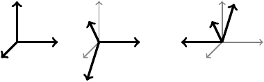
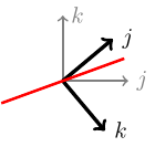
General nonsense says that this is again a rotation about some axis. The axis is the line "left alone". We can actually figure out where that line must be from this picture. The $x$–axis ends up "flipped". So any line that protrudes out from the $y-z$–plane (i.e. has non-trivial $x$–component) will end up in the opposite half of space. So the axis must lie in the $y-z$–plane. Let's draw just what the transformation does to the $y-z$–plane.

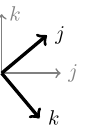
From this picture, we can see that what happens is that the $j$ and $k$ vectors are reflected in a line. That line is the bisector of where $j$ starts and ends up.

So the axis is $(0,\cos (\theta /2),\sin (\theta /2))$. The rotation angle is again $\pi$, whence this rotation is:

$$(\pi ,j)(\theta ,i)=(\pi ,0,\cos (\theta /2),\sin (\theta /2)).$$

Now let's try something a little more complicated. A rotation of $\theta$ about the $y$–axis followed by a rotation $\varphi$ about the $x$–axis. Where do we end up? General nonsense says that this is a rotation about some axis. The matrices for these are:

$$\left[\begin{array}{ccc}\cos (\theta )& 0& \sin (\theta )\\ 0& 1& 0\\ -\sin (\theta )& 0& \cos (\theta )\end{array}\right]\text{and}\left[\begin{array}{ccc}1& 0& 0\\ 0& \cos (\varphi )& -\sin (\varphi )\\ 0& \sin (\varphi )& \cos (\varphi )\end{array}\right]$$

Their product is:

$$\left[\begin{array}{ccc}1& 0& 0\\ 0& \cos (\varphi )& -\sin (\varphi )\\ 0& \sin (\varphi )& \cos (\varphi )\end{array}\right]\left[\begin{array}{ccc}\cos (\theta )& 0& \sin (\theta )\\ 0& 1& 0\\ -\sin (\theta )& 0& \cos (\theta )\end{array}\right]=\left[\begin{array}{ccc}\cos (\theta )& 0& \sin (\theta )\\ \sin (\varphi )\sin (\theta )& \cos (\varphi )& -\sin (\varphi )\cos (\theta )\\ -\cos (\varphi )\sin (\theta )& \sin (\varphi )& \cos (\varphi )\cos (\theta )\end{array}\right]$$

We want to know how to describe this as a rotation about some axis. The axis will be its "invariant vector". That is, $\stackrel{\rightharpoonup }{v}$ such that $A\stackrel{\rightharpoonup }{v}=\stackrel{\rightharpoonup }{v}$, or $(I-A)\stackrel{\rightharpoonup }{v}=\stackrel{\rightharpoonup }{0}$. We can find that vector using elementary linear algebra. We look at the matrix:

$$I-A=\left[\begin{array}{ccc}1-\cos (\theta )& 0& -\sin (\theta )\\ -\sin (\varphi )\sin (\theta )& 1-\cos (\varphi )& \sin (\varphi )\cos (\theta )\\ \cos (\varphi )\sin (\theta )& -\sin (\varphi )& 1-\cos (\varphi )\cos (\theta )\end{array}\right]$$

Knowing that $(I-A)\stackrel{\rightharpoonup }{v}=\stackrel{\rightharpoonup }{0}$ has a non-trivial solution, we can see that if we write a solution vector as $(x,y,z)$ then we have (from the top line):

$$x=\frac{\sin (\theta )}{1-\cos (\theta )}z$$

while from the middle line we have:

$$y=\frac{\sin (\varphi )}{1-\cos (\varphi )}(\sin (\theta )x-\cos (\theta )z).$$

Substituting in, we find that:

$$\begin{array}{rl}y& =\frac{\sin (\varphi )}{1-\cos (\varphi )}(\sin (\theta )\frac{\sin (\theta )}{1-\cos (\theta )}z-\cos (\theta )z)\\ & =\frac{z\sin (\varphi )}{(1-\cos (\varphi ))(1-\cos (\theta ))}({\sin }^2(\theta )-(1-\cos (\theta ))\cos (\theta ))\\ & =\frac{z\sin (\varphi )}{(1-\cos (\varphi ))(1-\cos (\theta ))}({\sin }^2(\theta )-\cos (\theta )+{\cos }^2(\theta ))\\ & =\frac{z\sin (\varphi )}{(1-\cos (\varphi ))(1-\cos (\theta ))}(1-\cos (\theta ))\\ & =\frac{z\sin (\varphi )}{1-\cos (\varphi )}\end{array}$$

We can simplify this a little by noting that the double angle formulae imply that:

$$\frac{\sin (\theta )}{1-\cos (\theta )}=\frac{2\sin (\theta /2)\cos (\theta /2)}{{\cos }^2(\theta /2)+{\sin }^2(\theta /2)-{\cos }^2(\theta /2)+{\sin }^2(\theta /2)}=\frac{2\sin (\theta /2)\cos (\theta /2)}{2{\sin }^2(\theta /2)}=\frac{\cos (\theta /2)}{\sin (\theta /2)}$$

So our invariant line is along the vector:

$$(\frac{\cos (\theta /2)}{\sin (\theta /2)},\frac{\cos (\varphi /2)}{\sin (\varphi /2)},1)$$

or, equivalently:

$$(\cos (\theta /2)\sin (\varphi /2),\cos (\varphi /2)\sin (\theta /2),\sin (\theta /2)\sin (\varphi /2)).$$

This isn't a unit vector so isn't right for an axis, but before we normalise it let us work out the angle of the new rotation. Looking at the two matrices for the simple rotations we see that the sum of the diagonal entries is $1+2\cos (\theta )$ and $1+2\cos (\varphi )$. This is true in general, so if we write the new angle as $\psi$ it will satisfy:

$$1+2\cos (\psi )=\cos (\theta )+\cos (\varphi )+\cos (\theta )\cos (\varphi ).$$

The right-hand side simplifies using double angle formulae as follows:

$$\begin{array}{rl}\cos (\theta )+\cos (\varphi )+\cos (\theta )\cos (\varphi )& =(1+\cos (\theta ))(1+\cos (\varphi ))-1\\ & =({\cos }^2(\theta /2)+{\sin }^2(\theta /2)+{\cos }^2(\theta /2)-{\sin }^2(\theta /2))(1+\cos (\varphi ))-1\\ & =2{\cos }^2(\theta /2)(1+\cos (\varphi /2))-1\\ & =4{\cos }^2(\theta /2){\cos }^2(\varphi /2)-1\\ & =(2\cos (\theta /2)\cos (\varphi /2){)}^2-1\end{array}$$

The left-hand side simplifies as:

$$\begin{array}{rl}1+2\cos (\psi )& ={\cos }^2(\psi /2)+{\sin }^2(\psi /2)+2{\cos }^2(\psi /2)-2{\sin }^2(\psi /2)\\ & =3{\cos }^2(\psi /2)-{\sin }^2(\psi /2)\\ & =4{\cos }^2(\psi /2)-({\cos }^2(\psi /2)+{\sin }^2(\psi /2))\\ & =(2\cos (\psi /2){)}^2-1.\end{array}$$

Hence (upto a sign ambiguity), the new angle is related to the old ones by the formula:

$$\cos (\psi /2)=\cos (\theta /2)\cos (\varphi /2).$$

Half angles are proving to be rather important! Although it isn't half angles that keep turning up, it is their sines and cosines. So instead of recording the angle and the axis maybe we can get away with recording the sine and cosine of the half angle together with the axis. Note that we can reconstruct the matrix from the sine and cosine of the half angles since the matrix only needs to know the sine and cosine of the full angle and we get that from the double angle formulae:

$$\begin{array}{rl}\cos (\theta )& ={\cos }^2(\theta /2)-{\sin }^2(\theta /2),\\ \sin (\theta )& =2\cos (\theta /2)\sin (\theta /2).\end{array}$$

This seems as though we are adding in another piece of information as we now record five numbers: $(\cos (\theta /2),\sin (\theta /2),\stackrel{\rightharpoonup }{v})$. However, although more information it is more useful in that the cosine and sine of the half angle is an easier starting point than the angle.

Expressed in these terms, our initial rules are:

$$\begin{array}{rl}(0,1,i)(0,1,j)& =(0,1,k)\\ (\alpha ,\beta ,\stackrel{\rightharpoonup }{v})(\gamma ,\delta ,\stackrel{\rightharpoonup }{v})& =(\alpha \gamma -\beta \delta ,\alpha \delta +\beta \gamma ,\stackrel{\rightharpoonup }{v})\\ (0,1,j)(\alpha ,\beta ,i)& =(0,1,\alpha j+\beta k)\end{array}$$

The final rule looks quite simple except for the fact that we haven't renormalised the axis. If we ignore that, we get:

$$(\alpha ,\beta ,i)(\gamma ,\delta ,j)=(\alpha \gamma ,?,\gamma \beta i+\alpha \delta j+\beta \delta k).$$

I put a question mark in there as I don't know what the sine of the half angle is. I could work it out, but I'd like to see if I can avoid it. That last formula is quite suggestive. Let me write it slightly differently. By complete abuse of notation, let me identify a unit vector in ${ℝ}^3$ with a half rotation about that axis. Thus we use $i$ to also mean the rotation $(\pi ,i)$. With this notation, our first rule reads $ij=k$. Putting this in to the above formula (this is where the real abuse of notation comes in) we get:

$$(\alpha ,\beta ,i)(\gamma ,\delta ,j)=(\alpha \gamma ,?,\gamma \beta i+\alpha \delta j+\beta \delta ij).$$

The thing to notice about this is that $i$ never appears except that $\beta$ is next to it, similarly $j$ always comes along with $\delta$. So if we are entertaining not normalising our axes (after all, is it really necessary?) we could write $(\alpha ,\beta ,\stackrel{\rightharpoonup }{v})$ as $(\alpha ,\beta \stackrel{\rightharpoonup }{v})$. Does this work? Let's try it with our rules.

$$\begin{array}{rl}(0,i)(0,j)& =(0,k)\\ (0,j)(\alpha ,\beta i)& =(0,\alpha j+(\beta i)j)\\ (\alpha ,\beta i)(\gamma ,\delta j)& =(\alpha \gamma ,\gamma (\beta i)+\alpha (\delta j)+(\beta i)(\delta j))\end{array}$$

The one we've left out this time is the second formula. In this one, let ${\stackrel{\rightharpoonup }{v}}_1=\beta \stackrel{\rightharpoonup }{v}$ and ${\stackrel{\rightharpoonup }{v}}_2=\delta \stackrel{\rightharpoonup }{v}$. Then the axis becomes $\alpha {\stackrel{\rightharpoonup }{v}}_2+\gamma {\stackrel{\rightharpoonup }{v}}_1$ which is fine. But the half angle is $\alpha \gamma -\beta \delta$ so we need to recover the product $\beta \delta$. As $\stackrel{\rightharpoonup }{v}$ is a unit vector, we can get this from ${\stackrel{\rightharpoonup }{v}}_1\cdot {\stackrel{\rightharpoonup }{v}}_2=\beta \delta \stackrel{\rightharpoonup }{v}\cdot \stackrel{\rightharpoonup }{v}=\beta \delta$. Thus our second rule is:

$$(\alpha ,{\stackrel{\rightharpoonup }{v}}_1)(\gamma ,{\stackrel{\rightharpoonup }{v}}_2)=(\alpha \gamma -{\stackrel{\rightharpoonup }{v}}_1\cdot {\stackrel{\rightharpoonup }{v}}_2,\alpha {\stackrel{\rightharpoonup }{v}}_2+\gamma {\stackrel{\rightharpoonup }{v}}_1).$$

6 The Product Rule

Let's look again at the rule:

$$(\alpha ,\beta i)(\gamma ,\delta j)=(\alpha \gamma ,\gamma (\beta i)+\alpha (\delta j)+(\beta i)(\delta j))$$

This looks a lot like the "product rule" for distributing multiplication over addition:

$$(a+b)(c+d)=ac+bc+ad+bd$$

Indeed, if we write the comma as a plus, we get precisely that:

$$(\alpha +\beta i)(\gamma +\delta j)=\alpha \gamma +\gamma (\beta i)+\alpha (\delta j)+(\beta i)(\delta j)$$

This case dealt with the situation where the two rotations have orthogonal axes. What about the opposite where the rotations have the same axis? Here we had:

$$(\alpha ,{\stackrel{\rightharpoonup }{v}}_1)(\gamma ,{\stackrel{\rightharpoonup }{v}}_2)=(\alpha \gamma -{\stackrel{\rightharpoonup }{v}}_1\cdot {\stackrel{\rightharpoonup }{v}}_2,\alpha {\stackrel{\rightharpoonup }{v}}_2+\gamma {\stackrel{\rightharpoonup }{v}}_1).$$

Can we make that fit the above pattern? We want to write:

$$(\alpha +{\stackrel{\rightharpoonup }{v}}_1)(\gamma +{\stackrel{\rightharpoonup }{v}}_2)=(\alpha \gamma -{\stackrel{\rightharpoonup }{v}}_1\cdot {\stackrel{\rightharpoonup }{v}}_2)+\alpha {\stackrel{\rightharpoonup }{v}}_2+\gamma {\stackrel{\rightharpoonup }{v}}_1$$

This works providing we accept that the "product" of two parallel axes should be the negative of their dot product.

So the product of two parallel axes is the negative of their dot product, and the product of two orthogonal axes is … what? For $i$ and $j$ it was $k$. Is there a general operation on vectors that for $i$ and $j$ spits out $k$? There is: the cross product. So for orthogonal axes we would expect to get the cross product.

Now given any two vectors, say $\stackrel{\rightharpoonup }{u}$ and $\stackrel{\rightharpoonup }{v}$, with $\stackrel{\rightharpoonup }{v}\ne \stackrel{\rightharpoonup }{0}$ we can write $\stackrel{\rightharpoonup }{u}=\lambda \stackrel{\rightharpoonup }{v}+\stackrel{\rightharpoonup }{w}$ where $\stackrel{\rightharpoonup }{w}$ is orthogonal to $\stackrel{\rightharpoonup }{v}$. Since multiplication ought to distribute over addition we would expect the following rule:

$$\stackrel{\rightharpoonup }{u}\stackrel{\rightharpoonup }{v}=(\lambda \stackrel{\rightharpoonup }{v}+\stackrel{\rightharpoonup }{w})\stackrel{\rightharpoonup }{v}=-\lambda \stackrel{\rightharpoonup }{v}\cdot \stackrel{\rightharpoonup }{v}+\stackrel{\rightharpoonup }{w}\times \stackrel{\rightharpoonup }{v}.$$

This simplifies since $\stackrel{\rightharpoonup }{w}\cdot \stackrel{\rightharpoonup }{v}=0$ and $\stackrel{\rightharpoonup }{v}\times \stackrel{\rightharpoonup }{v}=\stackrel{\rightharpoonup }{0}$, whence:

$$\begin{array}{rl}\stackrel{\rightharpoonup }{u}\cdot \stackrel{\rightharpoonup }{v}& =(\lambda \stackrel{\rightharpoonup }{v}+\stackrel{\rightharpoonup }{w})\cdot \stackrel{\rightharpoonup }{v}=\lambda \stackrel{\rightharpoonup }{v}\cdot \stackrel{\rightharpoonup }{v}\\ \stackrel{\rightharpoonup }{u}\times \stackrel{\rightharpoonup }{v}& =(\lambda \stackrel{\rightharpoonup }{v}+\stackrel{\rightharpoonup }{w})\times \stackrel{\rightharpoonup }{v}=\stackrel{\rightharpoonup }{w}\times \stackrel{\rightharpoonup }{v}\end{array}$$

whence

$$\stackrel{\rightharpoonup }{u}\stackrel{\rightharpoonup }{v}=-\stackrel{\rightharpoonup }{u}\cdot \stackrel{\rightharpoonup }{v}+\stackrel{\rightharpoonup }{u}\times \stackrel{\rightharpoonup }{v}.$$

Now none of this is a proof. We have no reason for believing that multiplication really does distribute over addition in this way. Also we have generalised from some very specific examples to the general case. Nonetheless, it is evidence for the following conjecture.

Conjecture Let $R_1$ be a rotation of angle ${\theta }_1$ about unit axis ${\stackrel{\rightharpoonup }{v}}_1$ and $R_2$ a rotation of angle ${\theta }_2$ about unit axis ${\stackrel{\rightharpoonup }{v}}_2$. Let $R_3=R_1{R}_2$ be their composition and let ${\theta }_3$ be its angle of rotation about axis ${\stackrel{\rightharpoonup }{v}}_3$.

For $r=1,2,3$ let ${\alpha }_r=\cos ({\theta }_r/2)$ and ${\stackrel{\rightharpoonup }{u}}_r=\sin ({\theta }_r/2){\stackrel{\rightharpoonup }{v}}_r$. Then:

$${\alpha }_3+{\stackrel{\rightharpoonup }{u}}_3=({\alpha }_1+{\stackrel{\rightharpoonup }{u}}_1)({\alpha }_2+{\stackrel{\rightharpoonup }{u}}_2)={\alpha }_1{\alpha }_2-{\stackrel{\rightharpoonup }{u}}_1\cdot {\stackrel{\rightharpoonup }{u}}_2+{\alpha }_1{\stackrel{\rightharpoonup }{u}}_2+{\alpha }_2{\stackrel{\rightharpoonup }{u}}_1+{\stackrel{\rightharpoonup }{u}}_1\times {\stackrel{\rightharpoonup }{u}}_2.$$

This rule certainly subsumes all of our previous rules, but for a proof we need to show that this works for any rotations. There is a geometric argument that says that it is enough to show this under certain assumptions on the axes, but it will be more useful for later if we work out the transformation matrix starting from the cosine of the half angle and the scaled axis.

So we start with a rotation with data $\alpha +\stackrel{\rightharpoonup }{u}$. The assumption is that $\alpha$ is the cosine of the half angle and $\stackrel{\rightharpoonup }{u}$ has been scaled by sine of the half angle. Note that under those assumptions,

$${\alpha }^2+\stackrel{\rightharpoonup }{u}\cdot \stackrel{\rightharpoonup }{u}={\cos }^2(\theta /2)+{\sin }^2(\theta /2)=1.$$

What is the resultant transformation? Let $\stackrel{\rightharpoonup }{v}$ be an arbitrary vector. Since rotations are linear, we can split $\stackrel{\rightharpoonup }{v}$ into a piece along the axis and a piece orthogonal to it:

$$\stackrel{\rightharpoonup }{v}=\frac{\stackrel{\rightharpoonup }{v}\cdot \stackrel{\rightharpoonup }{u}}{\stackrel{\rightharpoonup }{u}\cdot \stackrel{\rightharpoonup }{u}}\stackrel{\rightharpoonup }{u}+(\stackrel{\rightharpoonup }{v}-\frac{\stackrel{\rightharpoonup }{v}\cdot \stackrel{\rightharpoonup }{u}}{\stackrel{\rightharpoonup }{u}\cdot \stackrel{\rightharpoonup }{u}}\stackrel{\rightharpoonup }{u}).$$

The part along the axis stays the same. The part orthogonal rotates by the given angle. To specify this rotation we need two vectors in the orthogonal plane. Assuming that we weren't unlucky in our choice we already have one of them: the orthogonal part of $\stackrel{\rightharpoonup }{v}$. We can get another using cross products:

$$\stackrel{\rightharpoonup }{u}\times (\stackrel{\rightharpoonup }{v}-\frac{\stackrel{\rightharpoonup }{v}\cdot \stackrel{\rightharpoonup }{u}}{\stackrel{\rightharpoonup }{u}\cdot \stackrel{\rightharpoonup }{u}}\stackrel{\rightharpoonup }{u}).$$

This isn't quite the vector we'll use. For a start, we can simplify it:

$$\stackrel{\rightharpoonup }{u}\times (\stackrel{\rightharpoonup }{v}-\frac{\stackrel{\rightharpoonup }{v}\cdot \stackrel{\rightharpoonup }{u}}{\stackrel{\rightharpoonup }{u}\cdot \stackrel{\rightharpoonup }{u}}\stackrel{\rightharpoonup }{u})=\stackrel{\rightharpoonup }{u}\times \stackrel{\rightharpoonup }{v}-\frac{\stackrel{\rightharpoonup }{v}\cdot \stackrel{\rightharpoonup }{u}}{\stackrel{\rightharpoonup }{u}\cdot \stackrel{\rightharpoonup }{u}}\stackrel{\rightharpoonup }{u}\times \stackrel{\rightharpoonup }{u}=\stackrel{\rightharpoonup }{u}\times \stackrel{\rightharpoonup }{v}.$$

More importantly, it's the wrong length. We need our two orthogonal vectors to have the same length. That is, we want $\stackrel{\rightharpoonup }{u}\times \stackrel{\rightharpoonup }{v}$ to have the same length as $\stackrel{\rightharpoonup }{v}-\frac{\stackrel{\rightharpoonup }{v}\cdot \stackrel{\rightharpoonup }{u}}{\stackrel{\rightharpoonup }{v}\cdot \stackrel{\rightharpoonup }{v}}\stackrel{\rightharpoonup }{u}$. Since $\stackrel{\rightharpoonup }{u}$ is orthogonal to $\stackrel{\rightharpoonup }{v}-\frac{\stackrel{\rightharpoonup }{v}\cdot \stackrel{\rightharpoonup }{u}}{\stackrel{\rightharpoonup }{v}\cdot \stackrel{\rightharpoonup }{v}}\stackrel{\rightharpoonup }{u}$ the length of their cross product is the product of their lengths. Thus $\stackrel{\rightharpoonup }{u}\times \stackrel{\rightharpoonup }{v}$ is a factor of $\parallel \stackrel{\rightharpoonup }{u}\parallel$ out. So we take:

$$\stackrel{\rightharpoonup }{w}=\frac{1}{\parallel \stackrel{\rightharpoonup }{u}\parallel }\stackrel{\rightharpoonup }{u}\times \stackrel{\rightharpoonup }{v}$$

for our third vector.

The rotation rotates $\stackrel{\rightharpoonup }{v}-\frac{\stackrel{\rightharpoonup }{v}\cdot \stackrel{\rightharpoonup }{u}}{\stackrel{\rightharpoonup }{u}\cdot \stackrel{\rightharpoonup }{u}}\stackrel{\rightharpoonup }{u}$ by angle $\theta$ towards $\stackrel{\rightharpoonup }{w}$. Thus the total transformation is:

$$\begin{array}{rl}\stackrel{\rightharpoonup }{v}& \mapsto \frac{\stackrel{\rightharpoonup }{v}\cdot \stackrel{\rightharpoonup }{u}}{\stackrel{\rightharpoonup }{u}\cdot \stackrel{\rightharpoonup }{u}}\stackrel{\rightharpoonup }{u}+\cos (\theta )(\stackrel{\rightharpoonup }{v}-\frac{\stackrel{\rightharpoonup }{v}\cdot \stackrel{\rightharpoonup }{u}}{\stackrel{\rightharpoonup }{u}\cdot \stackrel{\rightharpoonup }{u}}\stackrel{\rightharpoonup }{u})+\sin (\theta )\stackrel{\rightharpoonup }{w}\\ & =\frac{\stackrel{\rightharpoonup }{v}\cdot \stackrel{\rightharpoonup }{u}}{\stackrel{\rightharpoonup }{u}\cdot \stackrel{\rightharpoonup }{u}}\stackrel{\rightharpoonup }{u}+\cos (\theta )(\stackrel{\rightharpoonup }{v}-\frac{\stackrel{\rightharpoonup }{v}\cdot \stackrel{\rightharpoonup }{u}}{\stackrel{\rightharpoonup }{u}\cdot \stackrel{\rightharpoonup }{u}}\stackrel{\rightharpoonup }{u})+\sin (\theta )\frac{1}{\parallel \stackrel{\rightharpoonup }{u}\parallel }\stackrel{\rightharpoonup }{u}\times \stackrel{\rightharpoonup }{v}\end{array}$$

Now let us recall the double angle formulae:

$$\begin{array}{rl}\cos (\theta )& ={\cos }^2(\theta /2)-{\sin }^2(\theta /2)={\alpha }^2-\stackrel{\rightharpoonup }{u}\cdot \stackrel{\rightharpoonup }{u}\\ \sin (\theta )& =2\sin (\theta /2)\cos (\theta /2)=2\parallel \stackrel{\rightharpoonup }{u}\parallel \alpha \end{array}$$

and substitute in:

$$\begin{array}{rl}\stackrel{\rightharpoonup }{v}& \mapsto \frac{\stackrel{\rightharpoonup }{v}\cdot \stackrel{\rightharpoonup }{u}}{\stackrel{\rightharpoonup }{u}\cdot \stackrel{\rightharpoonup }{u}}\stackrel{\rightharpoonup }{u}+({\alpha }^2-\stackrel{\rightharpoonup }{u}\cdot \stackrel{\rightharpoonup }{u})(\stackrel{\rightharpoonup }{v}-\frac{\stackrel{\rightharpoonup }{v}\cdot \stackrel{\rightharpoonup }{u}}{\stackrel{\rightharpoonup }{u}\cdot \stackrel{\rightharpoonup }{u}}\stackrel{\rightharpoonup }{u})+2\parallel \stackrel{\rightharpoonup }{u}\parallel \alpha \frac{1}{\parallel \stackrel{\rightharpoonup }{u}\parallel }\stackrel{\rightharpoonup }{u}\times \stackrel{\rightharpoonup }{v}\\ & =\frac{\stackrel{\rightharpoonup }{v}\cdot \stackrel{\rightharpoonup }{u}}{\stackrel{\rightharpoonup }{u}\cdot \stackrel{\rightharpoonup }{u}}\stackrel{\rightharpoonup }{u}+{\alpha }^2\stackrel{\rightharpoonup }{v}-{\alpha }^2\frac{\stackrel{\rightharpoonup }{v}\cdot \stackrel{\rightharpoonup }{u}}{\stackrel{\rightharpoonup }{u}\cdot \stackrel{\rightharpoonup }{u}}\stackrel{\rightharpoonup }{u}-(\stackrel{\rightharpoonup }{u}\cdot \stackrel{\rightharpoonup }{u})\stackrel{\rightharpoonup }{v}+(\stackrel{\rightharpoonup }{v}\cdot \stackrel{\rightharpoonup }{u})\stackrel{\rightharpoonup }{u}+2\alpha \stackrel{\rightharpoonup }{u}\times \stackrel{\rightharpoonup }{v}\end{array}$$

In there we have a term:

$$\frac{\stackrel{\rightharpoonup }{v}\cdot \stackrel{\rightharpoonup }{u}}{\stackrel{\rightharpoonup }{u}\cdot \stackrel{\rightharpoonup }{u}}\stackrel{\rightharpoonup }{u}-{\alpha }^2\frac{\stackrel{\rightharpoonup }{v}\cdot \stackrel{\rightharpoonup }{u}}{\stackrel{\rightharpoonup }{u}\cdot \stackrel{\rightharpoonup }{u}}\stackrel{\rightharpoonup }{u}=(1-{\alpha }^2)\frac{\stackrel{\rightharpoonup }{v}\cdot \stackrel{\rightharpoonup }{u}}{\stackrel{\rightharpoonup }{u}\cdot \stackrel{\rightharpoonup }{u}}\stackrel{\rightharpoonup }{u}$$

Recall that ${\alpha }^2+\stackrel{\rightharpoonup }{u}\cdot \stackrel{\rightharpoonup }{u}=1$, whence this simplifies to $(\stackrel{\rightharpoonup }{v}\cdot \stackrel{\rightharpoonup }{u})\stackrel{\rightharpoonup }{u}$. This leaves us with:

$$\stackrel{\rightharpoonup }{v}\mapsto 2(\stackrel{\rightharpoonup }{v}\cdot \stackrel{\rightharpoonup }{u})\stackrel{\rightharpoonup }{u}+({\alpha }^2-\stackrel{\rightharpoonup }{u}\cdot \stackrel{\rightharpoonup }{u})\stackrel{\rightharpoonup }{v}+2\alpha \stackrel{\rightharpoonup }{u}\times \stackrel{\rightharpoonup }{v}.$$

At first sight, this is not very enlightening. At second sight, it at least justifies the fact that we are specifying a rotation using the cosine of the half angle and a certain scale factor of the angle: only $\alpha$ and $\stackrel{\rightharpoonup }{u}$ appear in this formula from the rotation. It is also a reasonably concise formula: there are no complicated cosines or sines. But still that doesn't practically help us resolve our conjecture since composing this formula with another such will be quite messy. So while we could do it and try to rearrange to get the expected formula, we'll take a short cut.

Remember that we introduced some dodgy notation earlier in which we identified a unit vector with a half rotation about that axis. This fits with our new additive notation since a half rotation has angle $\pi$ and so the half angle of a half rotation is $\pi /2$, whence we're identifying the unit vector $\stackrel{\rightharpoonup }{w}$ with $\cos (\pi /2)+\sin (\pi /2)\stackrel{\rightharpoonup }{w}=0+\stackrel{\rightharpoonup }{w}$. So it's looking more reasonable by the minute! (Though still not justified.)

Let's see what happens under our multiplicative formula when the first rotation is of this form:

$$(\alpha +\stackrel{\rightharpoonup }{u})(0+\stackrel{\rightharpoonup }{w})=-\stackrel{\rightharpoonup }{u}\cdot \stackrel{\rightharpoonup }{w}+\alpha \stackrel{\rightharpoonup }{w}+\stackrel{\rightharpoonup }{u}\times \stackrel{\rightharpoonup }{w}.$$

Still not very enlightening. But if we remember from earlier this isn't enough. When we computed $(\pi ,j)(\theta ,i)$ then the result was a rotation of angle $\pi$ but the axis had mysteriously only rotated half as much as we wanted (this is where we got the inkling that half angles would be important). So we need to apply the rotation again. Or at least, apply some other rotation. The difference between the special case, of $(\pi ,j)(\theta ,i)$, and the above is that in our special case the axes were orthogonal. In the above that isn't (necessarily) the case and so we've ended up with a non-trivial angle: we have $-\stackrel{\rightharpoonup }{u}\cdot \stackrel{\rightharpoonup }{w}$ in the "angle" part. If we simply rotate again by the same angle about the same axis we'll have the same issue. We need some way to get rid of that term. The obvious way to do it is to rotate about $-\stackrel{\rightharpoonup }{u}$ since that will introduce a term $-(-\stackrel{\rightharpoonup }{u}\cdot \stackrel{\rightharpoonup }{w})=\stackrel{\rightharpoonup }{u}\cdot \stackrel{\rightharpoonup }{w}$ to cancel out. But if we do rotate the same angle but about $-\stackrel{\rightharpoonup }{u}$ we simply cancel out the rotation that we've already done. We need a cunning plan.

The cunning plan is to remember that rotations do not commute. So applying the new rotation on the left has a different effect to applying it on the right.

Let's see if this cunning plan is the outlier2.

$$(\alpha +\stackrel{\rightharpoonup }{u})(0+\stackrel{\rightharpoonup }{w})(\alpha -\stackrel{\rightharpoonup }{u})=(-\stackrel{\rightharpoonup }{u}\cdot \stackrel{\rightharpoonup }{w}+\alpha \stackrel{\rightharpoonup }{w}+\stackrel{\rightharpoonup }{u}\times \stackrel{\rightharpoonup }{w})(\alpha -\stackrel{\rightharpoonup }{u})$$

Let's write:

$$\begin{array}{rl}\beta & =-\stackrel{\rightharpoonup }{u}\cdot \stackrel{\rightharpoonup }{w}\\ \stackrel{\rightharpoonup }{p}& =\alpha \stackrel{\rightharpoonup }{w}+\stackrel{\rightharpoonup }{u}\times \stackrel{\rightharpoonup }{w}\end{array}$$

so that we want to compute:

$$(\beta +\stackrel{\rightharpoonup }{p})(\alpha -\stackrel{\rightharpoonup }{u})=\beta \alpha +\stackrel{\rightharpoonup }{p}\cdot \stackrel{\rightharpoonup }{u}+\alpha \stackrel{\rightharpoonup }{p}-\beta \stackrel{\rightharpoonup }{u}-\stackrel{\rightharpoonup }{p}\times \stackrel{\rightharpoonup }{u}$$

Then:

$$\begin{array}{rl}\beta \alpha +\stackrel{\rightharpoonup }{p}\cdot \stackrel{\rightharpoonup }{u}& =-\alpha \stackrel{\rightharpoonup }{u}\cdot \stackrel{\rightharpoonup }{w}+(\alpha \stackrel{\rightharpoonup }{w}+\stackrel{\rightharpoonup }{u}\times \stackrel{\rightharpoonup }{w})\cdot \stackrel{\rightharpoonup }{u}\\ & =-\alpha \stackrel{\rightharpoonup }{u}\cdot \stackrel{\rightharpoonup }{w}+\alpha \stackrel{\rightharpoonup }{w}\cdot \stackrel{\rightharpoonup }{u}+(\stackrel{\rightharpoonup }{u}\times \stackrel{\rightharpoonup }{w})\cdot \stackrel{\rightharpoonup }{u}\\ & =0.\\ \alpha \stackrel{\rightharpoonup }{p}-\beta \stackrel{\rightharpoonup }{u}-\stackrel{\rightharpoonup }{p}\times \stackrel{\rightharpoonup }{u}& =\alpha (\alpha \stackrel{\rightharpoonup }{w}+\stackrel{\rightharpoonup }{u}\times \stackrel{\rightharpoonup }{w})+(\stackrel{\rightharpoonup }{u}\cdot \stackrel{\rightharpoonup }{w})\stackrel{\rightharpoonup }{u}-(\alpha \stackrel{\rightharpoonup }{w}+\stackrel{\rightharpoonup }{u}\times \stackrel{\rightharpoonup }{w})\times \stackrel{\rightharpoonup }{u}\\ & ={\alpha }^2\stackrel{\rightharpoonup }{w}+\alpha \stackrel{\rightharpoonup }{u}\times \stackrel{\rightharpoonup }{w}+(\stackrel{\rightharpoonup }{u}\cdot \stackrel{\rightharpoonup }{w})\stackrel{\rightharpoonup }{u}-\alpha \stackrel{\rightharpoonup }{w}\times \stackrel{\rightharpoonup }{u}-(\stackrel{\rightharpoonup }{u}\times \stackrel{\rightharpoonup }{w})\times \stackrel{\rightharpoonup }{u}\\ & ={\alpha }^2\stackrel{\rightharpoonup }{w}+2\alpha \stackrel{\rightharpoonup }{u}\times \stackrel{\rightharpoonup }{w}+(\stackrel{\rightharpoonup }{u}\cdot \stackrel{\rightharpoonup }{w})\stackrel{\rightharpoonup }{u}-(\stackrel{\rightharpoonup }{u}\times \stackrel{\rightharpoonup }{w})\times \stackrel{\rightharpoonup }{u}\end{array}$$

which is looking very promising.

We just need to deal with that last term: $-(\stackrel{\rightharpoonup }{u}\times \stackrel{\rightharpoonup }{w})\times \stackrel{\rightharpoonup }{u}$. This is orthogonal to $\stackrel{\rightharpoonup }{u}\times \stackrel{\rightharpoonup }{w}$ and to $\stackrel{\rightharpoonup }{u}$. So long as $\stackrel{\rightharpoonup }{w}$ is not parallel to $\stackrel{\rightharpoonup }{u}$ (and if it were this term would be zero so we wouldn't be worrying about it), a vector orthogonal to $\stackrel{\rightharpoonup }{u}\times \stackrel{\rightharpoonup }{w}$ and to $\stackrel{\rightharpoonup }{u}$ is $\stackrel{\rightharpoonup }{w}-\frac{\stackrel{\rightharpoonup }{w}\cdot \stackrel{\rightharpoonup }{u}}{\stackrel{\rightharpoonup }{u}\cdot \stackrel{\rightharpoonup }{u}}\stackrel{\rightharpoonup }{u}$. Thus there is some number $\lambda$ such that:

$$-(\stackrel{\rightharpoonup }{u}\times \stackrel{\rightharpoonup }{w})\times \stackrel{\rightharpoonup }{u}=\lambda (\stackrel{\rightharpoonup }{w}-\frac{\stackrel{\rightharpoonup }{w}\cdot \stackrel{\rightharpoonup }{u}}{\stackrel{\rightharpoonup }{u}\cdot \stackrel{\rightharpoonup }{u}}\stackrel{\rightharpoonup }{u}).$$

To find $\lambda$ we can take dot products of everything in site with $\stackrel{\rightharpoonup }{w}$ to get:

$$-((\stackrel{\rightharpoonup }{u}\times \stackrel{\rightharpoonup }{w})\times \stackrel{\rightharpoonup }{u})\cdot \stackrel{\rightharpoonup }{w}=\lambda (\stackrel{\rightharpoonup }{w}-\frac{\stackrel{\rightharpoonup }{w}\cdot \stackrel{\rightharpoonup }{u}}{\stackrel{\rightharpoonup }{u}\cdot \stackrel{\rightharpoonup }{u}}\stackrel{\rightharpoonup }{u})\cdot \stackrel{\rightharpoonup }{w}.$$

The left hand side is a "triple product", $(\stackrel{\rightharpoonup }{a}\times \stackrel{\rightharpoonup }{b})\cdot \stackrel{\rightharpoonup }{c}$, and it is invariant under cyclic permutation of its factors. So we get:

$$-((\stackrel{\rightharpoonup }{u}\times \stackrel{\rightharpoonup }{w})\cdot (\stackrel{\rightharpoonup }{u}\times \stackrel{\rightharpoonup }{w}))=\lambda (\stackrel{\rightharpoonup }{w}\cdot \stackrel{\rightharpoonup }{w}-\frac{(\stackrel{\rightharpoonup }{w}\cdot \stackrel{\rightharpoonup }{u}{)}^2}{\stackrel{\rightharpoonup }{u}\cdot \stackrel{\rightharpoonup }{u}}).$$

The length of $\stackrel{\rightharpoonup }{u}\times \stackrel{\rightharpoonup }{w}$ is the length of $\stackrel{\rightharpoonup }{u}$ times by the length of the part of $\stackrel{\rightharpoonup }{w}$ orthogonal to $\stackrel{\rightharpoonup }{u}$. Thus:

$$\begin{array}{rl}(\stackrel{\rightharpoonup }{u}\times \stackrel{\rightharpoonup }{w})\cdot (\stackrel{\rightharpoonup }{u}\times \stackrel{\rightharpoonup }{w})& =(\stackrel{\rightharpoonup }{u}\cdot \stackrel{\rightharpoonup }{u})(\stackrel{\rightharpoonup }{w}-\frac{\stackrel{\rightharpoonup }{w}\cdot \stackrel{\rightharpoonup }{u}}{\stackrel{\rightharpoonup }{u}\cdot \stackrel{\rightharpoonup }{u}}\stackrel{\rightharpoonup }{u})\cdot (\stackrel{\rightharpoonup }{w}-\frac{\stackrel{\rightharpoonup }{w}\cdot \stackrel{\rightharpoonup }{u}}{\stackrel{\rightharpoonup }{u}\cdot \stackrel{\rightharpoonup }{u}}\stackrel{\rightharpoonup }{u})\\ & =(\stackrel{\rightharpoonup }{u}\cdot \stackrel{\rightharpoonup }{u})(\stackrel{\rightharpoonup }{w}\cdot \stackrel{\rightharpoonup }{w}-2\frac{(\stackrel{\rightharpoonup }{w}\cdot \stackrel{\rightharpoonup }{u}{)}^2}{\stackrel{\rightharpoonup }{u}\cdot \stackrel{\rightharpoonup }{u}}+\frac{(\stackrel{\rightharpoonup }{w}\cdot \stackrel{\rightharpoonup }{u}{)}^2}{\stackrel{\rightharpoonup }{u}\cdot \stackrel{\rightharpoonup }{u}})\\ & =(\stackrel{\rightharpoonup }{u}\cdot \stackrel{\rightharpoonup }{u})(\stackrel{\rightharpoonup }{w}\cdot \stackrel{\rightharpoonup }{w}-\frac{(\stackrel{\rightharpoonup }{w}\cdot \stackrel{\rightharpoonup }{u}{)}^2}{\stackrel{\rightharpoonup }{u}\cdot \stackrel{\rightharpoonup }{u}})\end{array}$$

Whence $\lambda =-\stackrel{\rightharpoonup }{u}\cdot \stackrel{\rightharpoonup }{u}$ and

$$-(\stackrel{\rightharpoonup }{u}\times \stackrel{\rightharpoonup }{w})\cdot \stackrel{\rightharpoonup }{u}=-\stackrel{\rightharpoonup }{u}\cdot \stackrel{\rightharpoonup }{u}(\stackrel{\rightharpoonup }{w}-\frac{\stackrel{\rightharpoonup }{w}\cdot \stackrel{\rightharpoonup }{u}}{\stackrel{\rightharpoonup }{u}\cdot \stackrel{\rightharpoonup }{u}}\stackrel{\rightharpoonup }{u})=(\stackrel{\rightharpoonup }{w}\cdot \stackrel{\rightharpoonup }{u})\stackrel{\rightharpoonup }{u}-(\stackrel{\rightharpoonup }{u}\cdot \stackrel{\rightharpoonup }{u})\stackrel{\rightharpoonup }{w}$$

Substituting back in,

$$\begin{array}{rl}\alpha \stackrel{\rightharpoonup }{p}-\beta \stackrel{\rightharpoonup }{u}-\stackrel{\rightharpoonup }{p}\times \stackrel{\rightharpoonup }{u}& ={\alpha }^2\stackrel{\rightharpoonup }{w}+2\alpha \stackrel{\rightharpoonup }{u}\times \stackrel{\rightharpoonup }{w}+(\stackrel{\rightharpoonup }{u}\cdot \stackrel{\rightharpoonup }{w})\stackrel{\rightharpoonup }{u}+(\stackrel{\rightharpoonup }{w}\cdot \stackrel{\rightharpoonup }{u})\stackrel{\rightharpoonup }{u}-(\stackrel{\rightharpoonup }{u}\cdot \stackrel{\rightharpoonup }{u})\stackrel{\rightharpoonup }{w}\\ & =({\alpha }^2-\stackrel{\rightharpoonup }{u}\cdot \stackrel{\rightharpoonup }{u})\stackrel{\rightharpoonup }{w}+2\alpha \stackrel{\rightharpoonup }{u}\times \stackrel{\rightharpoonup }{w}+2(\stackrel{\rightharpoonup }{u}\cdot \stackrel{\rightharpoonup }{w})\stackrel{\rightharpoonup }{u}\end{array}$$

Thus we have shown the following.

Theorem Let $R$ be a rotation with representation $\alpha +\stackrel{\rightharpoonup }{u}$. Then for a vector $\stackrel{\rightharpoonup }{v}$ we have:

$$R\stackrel{\rightharpoonup }{v}=((\alpha +\stackrel{\rightharpoonup }{u})(0+\stackrel{\rightharpoonup }{v}))(\alpha -\stackrel{\rightharpoonup }{v}).$$

This is almost enough to prove our conjecture. What we have is that if we have two rotations then (with the obvious notation):

$$R_1{R}_2\stackrel{\rightharpoonup }{v}=(({\alpha }_1+{\stackrel{\rightharpoonup }{u}}_1)((({\alpha }_2+{\stackrel{\rightharpoonup }{u}}_2)(0+\stackrel{\rightharpoonup }{v}))({\alpha }_2-{\stackrel{\rightharpoonup }{v}}_2)\left)\right)({\alpha }_1-{\stackrel{\rightharpoonup }{v}}_1).$$

What we need is:

$$R_1{R}_2\stackrel{\rightharpoonup }{v}=(({\alpha }_1+{\stackrel{\rightharpoonup }{u}}_1)({\alpha }_2+{\stackrel{\rightharpoonup }{u}}_2))(0+\stackrel{\rightharpoonup }{v})(({\alpha }_2-{\stackrel{\rightharpoonup }{v}}_2)({\alpha }_1-{\stackrel{\rightharpoonup }{v}}_1)).$$

The point here is that the multiplications are being applied in different orders. If we have three numbers, say $a,b,c$, and wish to find their product then we can multiply them in two ways (without changing their order): first multiply $a$ and $b$ and then multiply this product by $c$; or multiply $b$ and $c$ and then multiply this product by $a$. We write these as $(ab)c$ and $a(bc)$. That multiplication of numbers is associative says that it doesn't matter which route we took. We need to know that our new multiplication is similarly associative so that we can rebracket multiplications to suit our purposes. Then our conjecture would follow from our theorem.

Except that we do need one more thing. We also need to examine the interaction of the operation $(\alpha +\stackrel{\rightharpoonup }{v})\mapsto (\alpha -\stackrel{\rightharpoonup }{v})$ with multiplication.

7 Quaternions

Our "objects of interest" are of the form "number and vector". To correspond to a rotation, these need to satisfy some condition (namely that ${\alpha }^2+\stackrel{\rightharpoonup }{u}\cdot \stackrel{\rightharpoonup }{u}=1$). But our multiplication formula makes sense without that condition, so for the moment let's ignore it. Thus we are studying things of the form "number and vector" with a strange multiplication given by the formula:

$$({\alpha }_1+{\stackrel{\rightharpoonup }{u}}_1)({\alpha }_2+{\stackrel{\rightharpoonup }{u}}_2)={\alpha }_1{\alpha }_2-{\stackrel{\rightharpoonup }{u}}_1\cdot {\stackrel{\rightharpoonup }{u}}_2+{\alpha }_1{\stackrel{\rightharpoonup }{u}}_2+{\alpha }_2{\stackrel{\rightharpoonup }{u}}_1+{\stackrel{\rightharpoonup }{u}}_1\times {\stackrel{\rightharpoonup }{u}}_2.$$

In this case, "vector" means "$3$–vector". A "number and vector" is thus a $4$–vector. So we can simplify our notation by working in ${ℝ}^4$ and with $4$–vectors. We'll use letters in the neighbourhood of $q$ for $4$–vectors. We can promote a number to a $4$–vector by the identification $\alpha \mapsto (\alpha ,0,0,0)$ and a $3$–vector to a $4$–vector by $\stackrel{\rightharpoonup }{v}\mapsto (0,\stackrel{\rightharpoonup }{v})=(0,{\stackrel{\rightharpoonup }{v}}_x,{\stackrel{\rightharpoonup }{v}}_y,{\stackrel{\rightharpoonup }{v}}_z)$. Thus $\alpha +\stackrel{\rightharpoonup }{u}=(\alpha ,\stackrel{\rightharpoonup }{u})$.

What we want to establish are the properties of ${ℝ}^4$ with this new multiplication. To see what we are aiming for, consider multiplication of numbers. This satisfies quite a few nice properties:

1. It is associative: $(ab)c=a(bc)$

2. It is commutative: $ab=ba$

3. It has a unit: $1a=a=a1$

4. Non-zero numbers have inverses: $a{a}^{-1}=1=a^{-1}a$

5. It distributes over addition: $a(b+c)=ab+ac$, $(a+b)c=ac+bc$

Let's examine these for our new multiplication on ${ℝ}^4$. In actual fact, the best to start with is distributivity. This is because the formula for the multiplication involves lots of additions so it will be nice to know that we can split those up.

Let $p,q,r\in {ℝ}^4$ and write them as $p=\alpha +\stackrel{\rightharpoonup }{u}$, $q=\beta +\stackrel{\rightharpoonup }{v}$, and $r=\gamma +\stackrel{\rightharpoonup }{w}$. Consider $p(q+r)$:

$$\begin{array}{rl}p(q+r)& =(\alpha +\stackrel{\rightharpoonup }{u})((\beta +\gamma )+(\stackrel{\rightharpoonup }{v}+\stackrel{\rightharpoonup }{w}))\\ & =\alpha (\beta +\gamma )-\stackrel{\rightharpoonup }{u}\cdot (\stackrel{\rightharpoonup }{v}+\stackrel{\rightharpoonup }{w})+\alpha (\stackrel{\rightharpoonup }{v}+\stackrel{\rightharpoonup }{w})+(\beta +\gamma )\stackrel{\rightharpoonup }{u}+\stackrel{\rightharpoonup }{u}\times (\stackrel{\rightharpoonup }{v}+\stackrel{\rightharpoonup }{w})\\ & =\alpha \beta +\alpha \gamma -\stackrel{\rightharpoonup }{u}\cdot \stackrel{\rightharpoonup }{v}-\stackrel{\rightharpoonup }{u}\cdot \stackrel{\rightharpoonup }{w}+\alpha \stackrel{\rightharpoonup }{v}+\alpha \stackrel{\rightharpoonup }{w}+\beta \stackrel{\rightharpoonup }{u}+\gamma \stackrel{\rightharpoonup }{u}+\stackrel{\rightharpoonup }{u}\times \stackrel{\rightharpoonup }{v}+\stackrel{\rightharpoonup }{u}\times \stackrel{\rightharpoonup }{w}\\ & =(\alpha \beta -\stackrel{\rightharpoonup }{u}\cdot \stackrel{\rightharpoonup }{v}+\alpha \stackrel{\rightharpoonup }{v}+\beta \stackrel{\rightharpoonup }{u}+\stackrel{\rightharpoonup }{u}\times \stackrel{\rightharpoonup }{v})+(\alpha \gamma -\stackrel{\rightharpoonup }{u}\cdot \stackrel{\rightharpoonup }{w}+\alpha \stackrel{\rightharpoonup }{w}+\gamma \stackrel{\rightharpoonup }{u}+\stackrel{\rightharpoonup }{u}\times \stackrel{\rightharpoonup }{w})\\ & =pq+pr\end{array}$$

A similar argument establishes $(p+q)r=pr+qr$.

The next property that we shall tackle is the unit. We want $p$ such that $pq=q=qp$. Looking at the formula for the multiplication, we want $p=\alpha +\stackrel{\rightharpoonup }{u}$ such that:

$$\alpha \beta -\stackrel{\rightharpoonup }{u}\cdot \stackrel{\rightharpoonup }{v}+\alpha \stackrel{\rightharpoonup }{v}+\beta \stackrel{\rightharpoonup }{u}+\stackrel{\rightharpoonup }{u}\times \stackrel{\rightharpoonup }{v}=\beta +\stackrel{\rightharpoonup }{v}.$$

Looking at that, we want $\alpha \beta -\stackrel{\rightharpoonup }{u}\cdot \stackrel{\rightharpoonup }{v}=\beta$. This has to hold for any $\beta +\stackrel{\rightharpoonup }{v}$. Taking $\beta +\stackrel{\rightharpoonup }{v}=0+\stackrel{\rightharpoonup }{u}$, we get $\stackrel{\rightharpoonup }{u}\cdot \stackrel{\rightharpoonup }{u}=0$ whence $\stackrel{\rightharpoonup }{u}=\stackrel{\rightharpoonup }{0}$. Then we must have $\alpha =1$. Substituting in, we see that this does work. Hence the unit is $1+\stackrel{\rightharpoonup }{0}$. (We also need to check that this works when multiplied on the right. This is straightforward.)

What about inverses? In this case, for $p=\alpha +\stackrel{\rightharpoonup }{u}$ (and we might need some non-zero condition here), we want $q=\beta +\stackrel{\rightharpoonup }{v}$ such that:

$$\alpha \beta -\stackrel{\rightharpoonup }{u}\cdot \stackrel{\rightharpoonup }{v}+\alpha \stackrel{\rightharpoonup }{v}+\beta \stackrel{\rightharpoonup }{u}+\stackrel{\rightharpoonup }{u}\times \stackrel{\rightharpoonup }{v}=1+\stackrel{\rightharpoonup }{0}$$

How do we get that $\stackrel{\rightharpoonup }{0}$? Well, $\stackrel{\rightharpoonup }{u}\times \stackrel{\rightharpoonup }{v}$ is orthogonal to both $\stackrel{\rightharpoonup }{v}$ and $\stackrel{\rightharpoonup }{u}$ so getting $\alpha \stackrel{\rightharpoonup }{v}+\beta \stackrel{\rightharpoonup }{u}+\stackrel{\rightharpoonup }{u}\times \stackrel{\rightharpoonup }{v}=\stackrel{\rightharpoonup }{0}$ is impossible unless $\stackrel{\rightharpoonup }{v}\times \stackrel{\rightharpoonup }{u}=\stackrel{\rightharpoonup }{0}$. To do this, we need $\stackrel{\rightharpoonup }{u}$ and $\stackrel{\rightharpoonup }{v}$ parallel. That is, $\stackrel{\rightharpoonup }{v}=\lambda \stackrel{\rightharpoonup }{u}$ for some $\lambda \in ℝ$. Then to get $\stackrel{\rightharpoonup }{0}$ we must have $\alpha \lambda +\beta =0$. Looking at the number part, we want to have $\alpha \beta -\stackrel{\rightharpoonup }{u}\cdot \stackrel{\rightharpoonup }{v}=1$. Substituting in, we get $-\lambda {\alpha }^2-\lambda \stackrel{\rightharpoonup }{u}\cdot \stackrel{\rightharpoonup }{u}=1$, whence $\lambda =-({\alpha }^2+\stackrel{\rightharpoonup }{u}\cdot \stackrel{\rightharpoonup }{u}{)}^{-1}$.

Note that ${\alpha }^2+\stackrel{\rightharpoonup }{u}\cdot \stackrel{\rightharpoonup }{u}$ is the dot product of $\alpha +\stackrel{\rightharpoonup }{u}$ with itself when considered as a $4$–vector, and is thus non-zero if and only if $\alpha +\stackrel{\rightharpoonup }{u}$ is non-zero. Hence if $p=\alpha +\stackrel{\rightharpoonup }{u}$ is non-zero it has a multiplicative inverse and that inverse is given by:

$$p^{-1}=\frac{1}{p\cdot p}(\alpha -\stackrel{\rightharpoonup }{u}).$$

Notice from the above that if $p=\alpha +\stackrel{\rightharpoonup }{u}$ and we write $\alpha -\stackrel{\rightharpoonup }{u}$ as $\overline{p}$ then $p\overline{p}=p\cdot p$. Then $p^{-1}=\overline{p}/(p\cdot p)$. In particular, if $p\cdot p=1$ then $p^{-1}=\overline{p}$. The condition for $p$ to represent a rotation is $p\cdot p=1$ so $p\mapsto \overline{p}$ is potentially a useful thing to know about.

Before turning to associativity, let us deal with commutativity. This fails, as is easily seen by example:

$$ij=(0+i)(0+j)=i\times j=k,ji=(0+j)(0+i)=j\times i=-k.$$

But this is okay. We're using some of these vectors to represent rotations and we want multiplication to correspond to composition and composition of rotations is not commutative.

And so, at last, to associativity. Using distributivity of multiplication over addition we can reduce the problem to one where each of the terms is either a "pure number" or a "pure vector".

If one of them is a "pure number" then we can reduce the triple product to a binary product. This is because multiplication by a pure number corresponds to scalar multiplication:

$$\alpha (\beta +\stackrel{\rightharpoonup }{u})=\alpha \beta +\alpha \stackrel{\rightharpoonup }{u}$$

and from the formula for multiplication, it is clear that:

$$({\alpha }_1+{\stackrel{\rightharpoonup }{u}}_1)(\lambda {\alpha }_2+\lambda {\stackrel{\rightharpoonup }{u}}_2)=\lambda ({\alpha }_1{\alpha }_2-{\stackrel{\rightharpoonup }{u}}_1\cdot {\stackrel{\rightharpoonup }{u}}_2+{\alpha }_1{\stackrel{\rightharpoonup }{u}}_2+{\alpha }_2{\stackrel{\rightharpoonup }{u}}_1+{\stackrel{\rightharpoonup }{u}}_1\times {\stackrel{\rightharpoonup }{u}}_2).$$

(And similarly for multiplication on the right.) Thus multiplication is associative if one of the terms is a pure number.

We therefore just need to consider the case of pure vectors:

$$\begin{array}{rl}\stackrel{\rightharpoonup }{u}(\stackrel{\rightharpoonup }{v}\stackrel{\rightharpoonup }{w})& =\stackrel{\rightharpoonup }{u}(-\stackrel{\rightharpoonup }{v}\cdot \stackrel{\rightharpoonup }{w}+\stackrel{\rightharpoonup }{v}\times \stackrel{\rightharpoonup }{w})\\ & =\stackrel{\rightharpoonup }{u}\cdot (\stackrel{\rightharpoonup }{v}\times \stackrel{\rightharpoonup }{w})-(\stackrel{\rightharpoonup }{v}\cdot \stackrel{\rightharpoonup }{w})\stackrel{\rightharpoonup }{u}+\stackrel{\rightharpoonup }{u}\times (\stackrel{\rightharpoonup }{v}\times \stackrel{\rightharpoonup }{w})\\ (\stackrel{\rightharpoonup }{u}\stackrel{\rightharpoonup }{v})\stackrel{\rightharpoonup }{w}& =(-\stackrel{\rightharpoonup }{u}\cdot \stackrel{\rightharpoonup }{v}+\stackrel{\rightharpoonup }{u}\times \stackrel{\rightharpoonup }{v})\stackrel{\rightharpoonup }{w}\\ & =(\stackrel{\rightharpoonup }{u}\times \stackrel{\rightharpoonup }{v})\cdot \stackrel{\rightharpoonup }{w}-(\stackrel{\rightharpoonup }{u}\cdot \stackrel{\rightharpoonup }{v})\stackrel{\rightharpoonup }{w}+(\stackrel{\rightharpoonup }{u}\times \stackrel{\rightharpoonup }{v})\times \stackrel{\rightharpoonup }{w}.\end{array}$$

The pure number terms are the same since the triple product is invariant under cyclic permutation:

$$(\stackrel{\rightharpoonup }{u}\times \stackrel{\rightharpoonup }{v})\cdot \stackrel{\rightharpoonup }{w}=\stackrel{\rightharpoonup }{w}\cdot (\stackrel{\rightharpoonup }{u}\times \stackrel{\rightharpoonup }{v})=\stackrel{\rightharpoonup }{u}\cdot (\stackrel{\rightharpoonup }{v}\times \stackrel{\rightharpoonup }{w}).$$

So we just need to look at the vector parts.

Again using distributivity over addition and scalar multiplication, we can split it into cases where vectors are equal or orthogonal, and are of unit length.

• $\stackrel{\rightharpoonup }{v}$ orthogonal to $\stackrel{\rightharpoonup }{w}$.

  The vector part of $\stackrel{\rightharpoonup }{u}(\stackrel{\rightharpoonup }{v}\stackrel{\rightharpoonup }{w})$ simplifies to $\stackrel{\rightharpoonup }{u}\times (\stackrel{\rightharpoonup }{v}\times \stackrel{\rightharpoonup }{w})$. Moreover, $\{\stackrel{\rightharpoonup }{v},\stackrel{\rightharpoonup }{w},\stackrel{\rightharpoonup }{v}\times \stackrel{\rightharpoonup }{w}\}$ forms an oriented orthogonal basis.

  • $\stackrel{\rightharpoonup }{u}$ orthogonal to both.

    Then $\stackrel{\rightharpoonup }{u}$ is (up to sign) $\stackrel{\rightharpoonup }{v}\times \stackrel{\rightharpoonup }{w}$ and so the vector part of $\stackrel{\rightharpoonup }{u}(\stackrel{\rightharpoonup }{v}\stackrel{\rightharpoonup }{w})$ is $\stackrel{\rightharpoonup }{0}$.

    We have $\stackrel{\rightharpoonup }{u}\cdot \stackrel{\rightharpoonup }{v}=0$ so that part of the second vanishes, and then as $\stackrel{\rightharpoonup }{u}$ is (up to sign) $\stackrel{\rightharpoonup }{v}\times \stackrel{\rightharpoonup }{w}$, $\stackrel{\rightharpoonup }{u}\times \stackrel{\rightharpoonup }{v}$ is (up to sign) $\stackrel{\rightharpoonup }{w}$ and the cross product also vanishes.

    Thus both sides have vector part $\stackrel{\rightharpoonup }{0}$.

  • $\stackrel{\rightharpoonup }{u}=\stackrel{\rightharpoonup }{v}$.

    Then $\stackrel{\rightharpoonup }{u}\times (\stackrel{\rightharpoonup }{v}\times \stackrel{\rightharpoonup }{w})=-\stackrel{\rightharpoonup }{w}$ so the vector term of $\stackrel{\rightharpoonup }{u}(\stackrel{\rightharpoonup }{v}\stackrel{\rightharpoonup }{w})$ is $-\stackrel{\rightharpoonup }{w}$. Looking at $(\stackrel{\rightharpoonup }{u}\stackrel{\rightharpoonup }{v})\stackrel{\rightharpoonup }{w}$, we see that $\stackrel{\rightharpoonup }{u}\times \stackrel{\rightharpoonup }{v}=\stackrel{\rightharpoonup }{0}$ and $\stackrel{\rightharpoonup }{u}\cdot \stackrel{\rightharpoonup }{v}=1$ so we are also left with $-\stackrel{\rightharpoonup }{w}$.

  • $\stackrel{\rightharpoonup }{u}=\stackrel{\rightharpoonup }{w}$.

    Then $\stackrel{\rightharpoonup }{u}\times (\stackrel{\rightharpoonup }{v}\times \stackrel{\rightharpoonup }{w})=\stackrel{\rightharpoonup }{v}$. The dot product term in the second vanishes, and $\stackrel{\rightharpoonup }{u}\times \stackrel{\rightharpoonup }{v}=-\stackrel{\rightharpoonup }{v}\times \stackrel{\rightharpoonup }{w}$, whence $(\stackrel{\rightharpoonup }{u}\times \stackrel{\rightharpoonup }{v})\times \stackrel{\rightharpoonup }{w}=\stackrel{\rightharpoonup }{v}$.

• $\stackrel{\rightharpoonup }{v}=\stackrel{\rightharpoonup }{w}$.

  In this case the vector part of the first term is just $-\stackrel{\rightharpoonup }{u}$.

  • $\stackrel{\rightharpoonup }{u}$ orthogonal to $\stackrel{\rightharpoonup }{v}$.

    The dot product part of the second term is then zero, leaving just $(\stackrel{\rightharpoonup }{u}\times \stackrel{\rightharpoonup }{v})\times \stackrel{\rightharpoonup }{w}$. As $\stackrel{\rightharpoonup }{u}$ and $\stackrel{\rightharpoonup }{v}$ are orthogonal, $\{\stackrel{\rightharpoonup }{u},\stackrel{\rightharpoonup }{v},\stackrel{\rightharpoonup }{u}\times \stackrel{\rightharpoonup }{v}\}$ is an oriented orthogonal basis for ${ℝ}^3$. Then $(\stackrel{\rightharpoonup }{u}\times \stackrel{\rightharpoonup }{v})\times \stackrel{\rightharpoonup }{v}=-\stackrel{\rightharpoonup }{u}$, whence we have $-\stackrel{\rightharpoonup }{u}$ as the vector part of the second term.

  • $\stackrel{\rightharpoonup }{u}=\stackrel{\rightharpoonup }{v}=\stackrel{\rightharpoonup }{w}$.

    The cross product in the second term vanishes, and the dot product term is $-\stackrel{\rightharpoonup }{w}=-\stackrel{\rightharpoonup }{u}$.

This exhausts all the possibilities and associativity is shown.

There is one last property that we want to show. This is to relate $\overline{p}\overline{q}$ to $\overline{(pq)}$. It is a standard exercise to show that $(pq{)}^{-1}=q^{-1}{p}^{-1}$, so since $\overline{p}$ differs from $p^{-1}$ simply by a scalar, this shows that $\overline{p}\overline{q}=\overline{(qp)}$ (the case where one is zero is trivial).

We therefore have a multiplication on ${ℝ}^4$ that is associative, not commutative, unital, distributes over addition and scalar multiplication, and has multiplicative inverses for non-zero vectors. There is also an involution.

Definition ${ℝ}^4$ together with the above structure is called the space of quaternions, and written $ℍ$.

($\mathbb{Q}$ was already taken by the rationals.)

8 Conclusion

So a quaternion is a $4$–vector where we know about multiplication. Unit quaternions, that is quaternions with $q\overline{q}=1$, define rotations on ${ℝ}^3$. The implementation of this is to take a $3$–vector, $\stackrel{\rightharpoonup }{v}$, and promote it to a quaternion. Then to apply a quaternion compute $q\stackrel{\rightharpoonup }{v}\overline{q}$. Composition of rotations corresponds to multiplication of quaternions since:

$$q(p\stackrel{\rightharpoonup }{v}\overline{p})\overline{q}=(qp)\stackrel{\rightharpoonup }{v}(\overline{p}\overline{q})=(qp)\stackrel{\rightharpoonup }{v}\overline{(qp)}$$

Knowing the angle and axis, we can easily get the quaternion as $(\cos (\theta /2),\sin (\theta /2)\stackrel{\rightharpoonup }{v})$. Knowing the quaternion, we can get the matrix by computing its effect on the standard basis vectors: $q=(\alpha ,\stackrel{\rightharpoonup }{u})$ has the effect:

$${\stackrel{\rightharpoonup }{e}}_i\mapsto 2({\stackrel{\rightharpoonup }{e}}_i\cdot \stackrel{\rightharpoonup }{u})\stackrel{\rightharpoonup }{u}+({\alpha }^2-\stackrel{\rightharpoonup }{u}\cdot \stackrel{\rightharpoonup }{u}){\stackrel{\rightharpoonup }{e}}_i+2\alpha \stackrel{\rightharpoonup }{u}\times {\stackrel{\rightharpoonup }{e}}_i.$$

So if we write $q=(a,b,c,d)$, we get the following as columns of the matrix:

$$\begin{array}{rlrl}{\stackrel{\rightharpoonup }{e}}_1& \mapsto 2b\left[\begin{array}{c}b\\ c\\ d\end{array}\right]+(a^2-b^2-c^2-d^2)\left[\begin{array}{c}1\\ 0\\ 0\end{array}\right]+2a\left[\begin{array}{c}0\\ d\\ -c\end{array}\right]& & =\left[\begin{array}{c}{a}^2+b^2-c^2-d^2\\ 2bc+2ad\\ 2bd-2ac\end{array}\right]\\ {\stackrel{\rightharpoonup }{e}}_2& \mapsto 2c\left[\begin{array}{c}b\\ c\\ d\end{array}\right]+(a^2-b^2-c^2-d^2)\left[\begin{array}{c}0\\ 1\\ 0\end{array}\right]+2a\left[\begin{array}{c}-d\\ 0\\ b\end{array}\right]& & =\left[\begin{array}{c}2cb-2ad\\ a^2-b^2+c^2-d^2\\ 2cd+2ab\end{array}\right]\\ {\stackrel{\rightharpoonup }{e}}_3& \mapsto 2d\left[\begin{array}{c}b\\ c\\ d\end{array}\right]+(a^2-b^2-c^2-d^2)\left[\begin{array}{c}0\\ 0\\ 1\end{array}\right]+2a\left[\begin{array}{c}c\\ -b\\ 0\end{array}\right]& & =\left[\begin{array}{c}2bd+2ac\\ 2dc-2ab\\ a^2-b^2-c^2+d^2\end{array}\right]\end{array}$$

The trickiest part is to go from the matrix to the quaternion. The angle comes from the trace. Recall that if $R$ is a rotation then the trace of $R$, the sum of the diagonal entries, is $1+2\cos (\theta )$. Taking the trace of the matrix from the quaternion above, we get:

$$3a^2-b^2-c^2-d^2=3a^2-(1-a^2)=4a^2-1.$$

Up to sign, this gives us $a$. Then we can read off $b,c,d$ using various entries of the matrix:

$$\begin{array}{rl}{R}_{21}-R_{12}& =2cb+2ad-(2bc-2ad)=4ad\\ R_{13}-R_{31}& =2bd+2ac-(2bd-2ac)=4ac\\ R_{32}-R_{23}& =2cd+2ab-(2dc-2ab)=4ab\end{array}$$

Note that we only get the quaternion up to a sign ambiguity.

9 Loose Ends

There are two loose ends to tie up:

1. What about a rotation of angle $0$?

2. How many representations do we have per genuine rotation?

The first is easily dealt with. A rotation of angle $0$ can be about any axis so in the "angle and axis" representation we have $(0,\stackrel{\rightharpoonup }{v})$ for any unit vector $\stackrel{\rightharpoonup }{v}$. But when we translate this into quaternions, we need to multiply $\stackrel{\rightharpoonup }{v}$ by $\sin (\theta /2)=\sin (0)=0$. So our representation for a rotation of angle $0$ is $(\cos (0),\sin (0)\stackrel{\rightharpoonup }{v})=(1,\stackrel{\rightharpoonup }{0})$.

The second is not quite so simple. The fact that we keep dividing angles by $2$ actually means that we end up with two representations per rotation. If we forgot that a rotation of $2\pi$ got us back where we started then we might be tempted to encode a rotation of $2\pi$ as $(2\pi ,\stackrel{\rightharpoonup }{v})$ which maps to $(\cos (\pi ),\sin (\pi )\stackrel{\rightharpoonup }{v})=(-1,\stackrel{\rightharpoonup }{0})$. And in fact, that works: if $q=(-1,\stackrel{\rightharpoonup }{0})$ then $q\stackrel{\rightharpoonup }{u}\overline{q}=\stackrel{\rightharpoonup }{v}$ so this is another encoding of the trivial rotation.

More generally, $q$ and $-q$ encode the same rotation since:

$$(-q)\stackrel{\rightharpoonup }{u}\overline{(-q)}=-q\stackrel{\rightharpoonup }{u}(-\overline{q})=q\stackrel{\rightharpoonup }{u}\overline{q}.$$

In technical terms the unit quaternions provide a double cover of the space of rotations. This only proves problematic if working globally with rotations. If one restricts to a small patch of axes and angles then this issue introduces no difficulties: given a particular quaternion $q$ with rotation $R_q$, there is a $1-1$ correspondence between quaternions near $q$ and rotations near $R_q$.

Where one needs to be aware of this is if one takes a path of rotations that "goes all the way around". The corresponding path of quaternions will only go half way around.

This doubling is related to the half angles and the fact that when we rotate an axis by a rotation we actually only rotate it by half the angle we thought we were rotating it by. Thus the unit quaternions are really acting not on points but on points with spin and when we rotate a point with spin all the way around the circle it, the axis only rotates half as much.

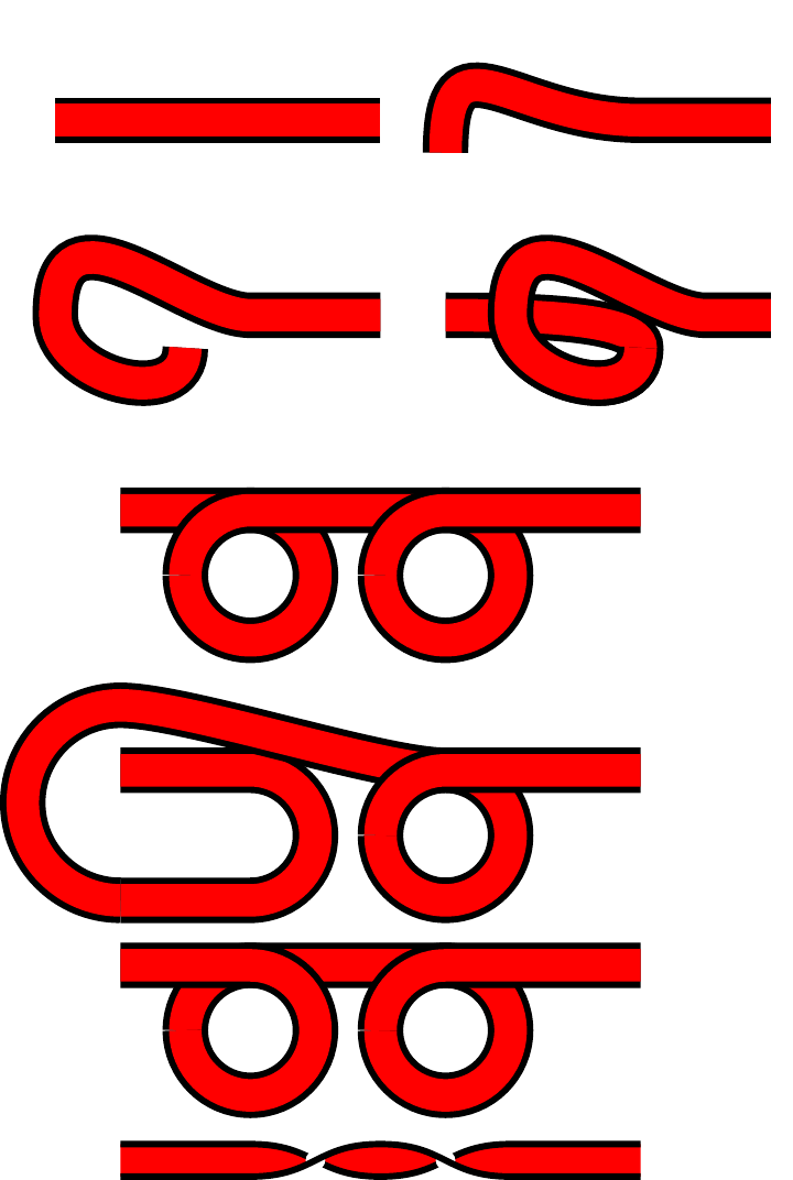
To go further in this vein would lead us to talk of spinors and fermions. Rather than going there, let me end with an alternative view of this doubling. Imagine attaching your point of interest by a ribbon to a "point at infinity". Now rotate it a full circle around the origin (with the rotation only affecting the ribbon by moving its end point, and at the crossing point we can lift the ribbon to let the point pass underneath). The ribbon is twisted. Do it again. The ribbon is still twisted. But now it is possible to untwist the ribbon without moving its endpoints.

Try it.

10 Why Bother?

The above explains what the quaternions are and aims to justify their role as an encoding scheme for rotations of $3$–space. However, it is somewhat light on why one would use them and how to best do so.

The "Why?" question is comparative. The assumption is that one wants to use rotations in some fashion and so one needs an encoding scheme. Thus "Why use quaternions?" is really "Why use quaternions as opposed to XYZ?". Let's compare a few different schemes:

1. Quaternions

2. Matrices

3. Angle and axis

4. Rotations about the major axes

Here are some salient facts:

1. Number of pieces of information to specify a rotation:

   1. Quaternions: $4$ numbers

   2. Matrices: $9$ numbers

   3. Angle and axis: $4$ numbers

   4. Rotations about the major axes: $3$ numbers

2. Computation of composition:

   1. Quaternions: $16$ multiplications, $12$ additions, $4$ assignments

   2. Matrices: $27$ multiplications, $18$ additions, $9$ assignments

   3. Angle and axis: Complicated! Involves cosine and sine of the angles involved.

   4. Rotations about the major axes: Complicated! Involves cosine and sine of the angles involved.

3. Computation of effect:

   1. Quaternions: $32$ multiplications, $24$ additions, $8$ assignments (in a lazy implementation)

   2. Matrices: $9$ multiplications, $6$ additions, $3$ assignments.

   3. Angle and axis: Involves sine and cosine of the angle involved.

   4. Rotations about the major axes: Involves sine and cosine of the angles involved.

4. Robustness:

   1. Quaternions: Very robust; any non-zero quaternion can be rescaled to a unit quaternion so a minor variation in the numbers can easily be corrected.

   2. Matrices: Not robust; it is possible to retract "all matrices" (well, half of all invertible matrices to be precise) onto the rotation matrices but the standard method for doing so is complicated and involves eigenvectors.

   3. Angle and axis: Very robust; any non-zero vector defines an axis.

   4. Rotations about the major axes: Very robust.

5. Ambient space:

   1. Quaternions: ambient space of unit quaternions is all quaternions, a skew-field.

   2. Matrices: ambient space of rotation matrices is all matrices, this is an algebra.

   3. Angle and axis: ambient space of axes is $3$–space, a vector space.

   4. Rotations about the major axes: no ambient space.

The ambient space is an important point. Rotations themselves have some structure but other than composition the structure is hard to use. Embedding them in some ambient space allows us access to all the structure of that ambient space. The catch is that using it might take us out of the space of rotations, but if there is a simple way to get back again then it can still be worth doing.

As an example, consider the problem of defining a path of rotations. Suppose we want to get from $R_1$ to $R_2$, but have no particular requirements on the path. With quaternions we can plan as follows: represent these as $q_1$ and $q_2$ and assume (without loss of generality) that $q_1\ne -q_2$. Then in $ℍ$ we can take the path $t\mapsto (1-t)q_1+t{q}_2$. This goes from $q_1$ at $t=0$ to $q_2$ at $t=1$. Unfortunately, it probably does not consist of unit quaternions (and thus rotations). Fortunately, we can simply renormalise as we go along to fix this. (The assumption that $q_1\ne -q_2$ ensures that we never go through the origin.) Doing the same thing with matrices is far more complicated: the projection from all suitable matrices to rotation matrices is more complicated to implement, and the space of matrices where this projection is defined is not as nice as "all non-zero quaternions".

Therefore, quaternions beat all other representations except in the application of a quaternion to a vector where matrices are better3.

So the answer to the question "Why should I use quaternions for rotations?" is that if you intend to do anything more than just apply the rotation, quaternions make life easier and more robust.

11 How To Use Quaternions

At a very basic level, quaternions are easy to use. Once you have a library (such as mine) that implements the standard quaternionic structure, all the tools are there for using quaternions to represent rotations.

Quaternions are simply an encoding scheme for rotations so when using quaternions one should always break down the problem into two:

1. What do I want to do to the rotations?

2. How do I do that using quaternions?

In other words, a conceptual and a practical part. Moreover, once the conceptual is sorted out the practical side is generally quite straightforward. So the "How?" of quaternions theoretically should not be a difficult question.

However, what happens in practice rarely follows the theoretical. And whilst quaternions themselves should present no conceptual issues, their use often serves to highlight conceptual problems with rotations themselves. So let's take a couple of uses of rotations that go a bit beyond the basics and see how to encode them using quaternions.

The two examples are the following:

1. Use touch events to rotate the view.

2. Use the iPad's orientation information to rotate the view.

In both cases, we shall work by adjusting the arguments to the camera function. We shall start with the frame set up so that we are looking at the origin from a point along the positive $z$–axis with the $y$–axis as "up". To give us something to look at we put a mesh at the origin.

11.1 Moving By Touch

We're looking at the origin and want to rotate the scene by touching the screen. There are various ways to make this work; the following method is based on imagining that there is a transparent sphere between the camera and what it is looking at. When we touch the screen of the iPad it is as if we move that sphere around.

We shall assume that the sphere is roughly the size of the iPad screen. So when you touch the iPad screen, you are touching a point on the sphere above the point you think you are touching. Providing the camera is "far" from the sphere, we can use orthogonal projection to find this point (if the camera is "near" we should use a stereographic projection but complete accuracy is not a high priority here).

We touch the screen at $\stackrel{\rightharpoonup }{t}$. This is relative to the bottom left of the screen, so we adjust its origin. We also normalise so that the sphere is of unit radius (this is because we are in search of a radius so our calculations are "scale invariant"). Thus we set $\stackrel{\rightharpoonup }{s}=(\stackrel{\rightharpoonup }{t}-\stackrel{\rightharpoonup }{o})/r$ where $\stackrel{\rightharpoonup }{o}$ is the centre of the screen and $r$ the radius of the sphere (whichever is the least of the width or height of the screen). Now, our calculations will go a bit wrong if we get too close to the "edge" of the sphere so we only proceed if $\parallel s\parallel <.9$. Our point on the sphere is then $\stackrel{\rightharpoonup }{S}=(s_x,s_y,\sqrt{1-s_x^2-s_y^2})$.

We now move to a new point. As before, we shift and scale this point, and let's write $\stackrel{\rightharpoonup }{e}$ for the result. As before, we set $\stackrel{\rightharpoonup }{E}=(e_x,e_y,\sqrt{1-e_x^2-e_y^2})$.

The problem is now to specify a rotation (in terms of a quaternion) that takes the point $\stackrel{\rightharpoonup }{S}$ to the point $\stackrel{\rightharpoonup }{E}$. As stated, this is not uniquely determined. We could arbitrarily rotate around $\stackrel{\rightharpoonup }{S}$ before doing the rotation to $\stackrel{\rightharpoonup }{E}$. So we add in the constraint that it should move space as little as possible. This means that we want the rotation in the plane of $\stackrel{\rightharpoonup }{S}$ and $\stackrel{\rightharpoonup }{E}$, so our axis is orthogonal to $\stackrel{\rightharpoonup }{S}$ and $\stackrel{\rightharpoonup }{E}$. The way to generate a vector orthogonal to two other vectors is to take their cross product so we set $\stackrel{\rightharpoonup }{u}=\stackrel{\rightharpoonup }{S}\times \stackrel{\rightharpoonup }{E}$.

The naïve way to proceed would be to normalise this axis, then figure out the angle, and feed that into the quaternion machine to find the rotation. However, we don't need to do all of that. If we let $\theta$ be the angle between $\stackrel{\rightharpoonup }{S}$ and $\stackrel{\rightharpoonup }{E}$ and let $\stackrel{\rightharpoonup }{w}$ be the unit vector in the direction of $\stackrel{\rightharpoonup }{u}$ then it turns out that $\stackrel{\rightharpoonup }{u}=\sin (\theta )\stackrel{\rightharpoonup }{w}$. Now, we actually want $\sin (\theta /2)$ but we're not far off. We also have $\cos (\theta )=\stackrel{\rightharpoonup }{S}\cdot \stackrel{\rightharpoonup }{E}$. Now the double angle formula gives us that $\cos (\theta )=2{\cos }^2(\theta /2)-1$, thus we can set $a=\sqrt{\stackrel{\rightharpoonup }{S}\cdot \stackrel{\rightharpoonup }{E}/2+1/2}$ (we can take the positive square root as it is a safe bet that $\theta$ is quite small). The other double angle formula says that $\sin (\theta )=2\sin (\theta /2)\cos (\theta /2)$ so $\sin (\theta /2)\stackrel{\rightharpoonup }{w}=\stackrel{\rightharpoonup }{u}/(2a)$.

Hence our quaternion is: $(a,\stackrel{\rightharpoonup }{S}\times \stackrel{\rightharpoonup }{E}/(2a))$ where $a=\sqrt{\stackrel{\rightharpoonup }{S}\cdot \stackrel{\rightharpoonup }{E}/2+1/2}$.

Note the distinct absence of cosines and sines. The most complicated operation being square roots.

An alternative method would be to take the bisector of $\stackrel{\rightharpoonup }{S}$ and $\stackrel{\rightharpoonup }{E}$. This is the renormalisation of $\stackrel{\rightharpoonup }{S}+\stackrel{\rightharpoonup }{E}$. Let's call this $\stackrel{\rightharpoonup }{B}$. The point of that is that the angle between $\stackrel{\rightharpoonup }{S}$ and $\stackrel{\rightharpoonup }{B}$ is $\theta /2$ so $\cos (\theta /2)=\stackrel{\rightharpoonup }{S}\cdot \stackrel{\rightharpoonup }{B}$, moreover the cross product of $\stackrel{\rightharpoonup }{S}$ and $\stackrel{\rightharpoonup }{B}$ is in the same direction as that of $\stackrel{\rightharpoonup }{S}$ and $\stackrel{\rightharpoonup }{E}$ but with length $\sin (\theta /2)$. This passes off the computation of the square root from the computation of the angle to the renormalisation of $\stackrel{\rightharpoonup }{S}+\stackrel{\rightharpoonup }{E}$. However, we can be a little sneaky, at the expense of a little accuracy. Instead of computing the bisector of $\stackrel{\rightharpoonup }{S}$ and $\stackrel{\rightharpoonup }{E}$, we can compute the midpoint of $\stackrel{\rightharpoonup }{s}$ and $\stackrel{\rightharpoonup }{e}$, say $\stackrel{\rightharpoonup }{b}$. So long as everything is small, the point on the sphere above $\stackrel{\rightharpoonup }{b}$ will be roughly the bisector of $\stackrel{\rightharpoonup }{S}$ and $\stackrel{\rightharpoonup }{E}$. Then our quaternion is $(\stackrel{\rightharpoonup }{S}\cdot \stackrel{\rightharpoonup }{B},\stackrel{\rightharpoonup }{S}\times \stackrel{\rightharpoonup }{B})$.

The last thing to note is that we actually want the inverse of this quaternion. This is because we are actually applying our transformation to the camera and not to the world inside. Thus we are not actually turning the sphere, rather we are moving ourselves around on (or relative to) the sphere's surface.

To conclude this section, let's extract a useful nugget. The problem is to rotate space so that a line, say $L_1$, ends up at, say, $L_2$. The strategy is as follows. Pick unit vectors, ${\stackrel{\rightharpoonup }{v}}_1$ along $L_1$ and ${\stackrel{\rightharpoonup }{v}}_2$ along $L_2$. Compute ${\stackrel{\rightharpoonup }{v}}_1+{\stackrel{\rightharpoonup }{v}}_2$. If it is non-zero, renormalise to $\stackrel{\rightharpoonup }{b}$. If not, let $\stackrel{\rightharpoonup }{b}$ be an arbitrary vector orthogonal to ${\stackrel{\rightharpoonup }{v}}_1$. Then the quaternion for the rotation is $({\stackrel{\rightharpoonup }{v}}_1\cdot \stackrel{\rightharpoonup }{b},{\stackrel{\rightharpoonup }{v}}_1\times \stackrel{\rightharpoonup }{b})$.

11.2 Moving By iPad

One of the great things about an iPad is the ability to pick it up and move it. In Codea 1.4, we can partially detect how an iPad is being held by examining the Gravity vector. With Codea 1.5 we also get access to the RotationRate.

Let's start with just Codea 1.4. The task here is to rotate the coordinate system so that the $y$–axis is always true vertical. This is not sufficiently specified, so to make it so we also require the $x$–axis to lie in the iPad screen. There will be certain orientations where this is still not sufficiently precise (namely, when the iPad is held horizontal) but for all else it will do.

Assuming that the $y$–axis is not parallel to the gravity vector, we can proceed as before since we want to move the $y$–axis to the gravity vector. Let us write $\stackrel{\rightharpoonup }{g}$ for the gravity vector, then we compute the bisector, say $\stackrel{\rightharpoonup }{b}$, as the renormalisation of $\stackrel{\rightharpoonup }{g}+(0,-1,0)$. Then $(0,-1,0)\cdot \stackrel{\rightharpoonup }{b}=-b_y$ and $(0,-1,0)\times \stackrel{\rightharpoonup }{b}=(-b_z,0,b_x)$.

Once again we need the inverse rotation.

This simply rotates the $y$–axis to where we want it. We also need to rotate around the $y$–axis to get the $x$–axis into the iPad screen. To do this, we need to know the vector in the screen that is orthogonal to the gravity vector. This is (up to scale) $(-g_y,g_x,0)$. So we rotate to get the $x$–axis to point in this direction, using the above method: set $\stackrel{\rightharpoonup }{b}=(-g_y,g_x,0)$, normalise, add $(1,0,0)$, normalise, and then get the quaternion which will be $(b_x,0,0,b_y)$ (assuming we storing the result in $\stackrel{\rightharpoonup }{b}$).

Now here's where it gets complicated. We have two rotations to apply. The first thing to note is that the order in which we apply them matters. The second thing to note is that we've computed each one with respect to the standard reference frame. But once we apply one rotation we need to ensure that the second is with respect to the new reference frame.

Let's rotate the $x$–axis first. Let $q$ be the resultant quaternion. Now $q$ represents a rotation of space and it has been designed so that it takes the model's frame of reference to the screen's frame of reference. That is, $(1,0,0{)}^q$ is where the model's $x$–axis will end up on screen.

(I've sneaked in some notation there. Often when something like quaternions acts on something different, like vectors, we write the action simply like multiplication: $x\mapsto gx$. But in this case that is ambiguous since we it makes sense to multiply a quaternion by a vector by thinking of the vector as a quaternion. To avoid this ambiguity, we use the alternative exponential notation for action: $x\mapsto x^g$. Thus ${\stackrel{\rightharpoonup }{v}}^q=q\stackrel{\rightharpoonup }{v}\overline{q}$.)

The second rotation is designed to take the $y$–axis to be parallel to the gravity vector. We're applying this after the first one. The key point here is that $y$–axis that we are working with is the model's $y$–axis. This isn't the current $y$–axis, which is the screen's $y$–axis. Rather it is $(0,1,0{)}^q$. So our second rotation takes $(0,1,0{)}^q$ to the gravity vector. (Or rather, $(0,-1,0{)}^q$ since we want gravity to be downwards.)

11.3 Combining the Two

We now have two sources of rotation: the tilt of the iPad and the touch data. We want to put the two together. But in which order?

To do this we need to work out what the user will expect. My assumption is that the user will expect that when they turn the object using touch, then they are genuinely turning the object. However, when tilting the iPad they are turning their view of the object. So the touch data needs to be "innermost". That is to say, our total rotation needs to be $R_g{R}_t$.

But there is a snag here. The actual touch data is relative to the screen. That is, when the user touches the screen then the new information is relative to the outermost set of coordinates. So we need to transform it into the innermost by conjugating it by the gravity rotation. Thus when the user touches the screen, we need to update the rotation matrix by $R_t\mapsto R_g^{-1}{R}_{\delta t}{R}_g{R}_t$.

Now notice what happens when we put that together with $R_g$ (with $R_{t\text{'}}$ being the "old" rotation):

$$R_g{R}_t=R_g{R}_g^{-1}{R}_{\delta t}{R}_g{R}_{t\text{'}}=R_{\delta t}{R}_g{R}_{t\text{'}}$$

So $R_{\delta t}$ is actually being applied relative to the screen coordinates as it should. The point is that the $R_g$ used in updating $R_t$ is then "frozen" at the time of updating. Then if the iPad is tilted further, so that $R_g$ changes, the above simplification no longer holds. Thus $R_{\delta t}$ is always relative to the screen coordinates that were in effect when the touch occurred.

11.4 Using Rotation Rate

With Codea 1.5 comes the RotationRate vector. Although a vector, it represents a rotation. The three components are the rotations that the iPad felt around its major axes. Technically, these are Tait-Bryan angles because they use three different axes, though they are sometimes referred to as Euler angles or yaw, pitch, and roll.

The units of RotationRate are radians per second. Thus we can convert each angle to a quaternion rotating around the given axis. This is the "instantaneous" rotation and is relative to the current screen coordinates, so we need to keep a running total to keep track of how the iPad moves. Thus each frame we need to do:

$$q\mapsto q_z{q}_y{q}_{x}q$$

where, for example, $q_x=(\cos ({\rho }_x\Delta t/2),\sin ({\rho }_x\Delta t/2),0,0)$.

One obvious question is as to the order in which to multiply the rotations, since the order matters. The best way to figure this out is to test it: try all six possibilities. Have Codea compute all six possibilities and to display the resulting quaternions. Then place the iPad in a known orientation and start the program. Rotate the iPad freely and wildly (making sure not just to rotate around the principal axes) and return it to the known state. The one that is closest to $(1,0,0,0)$ is the right order.

My tests show that $q_z{q}_y{q}_x$ is right.

However, as it is cumulative, inaccuracies will build up and so it should not be relied upon to give a truly accurate portrayal of the orientation of the iPad.

A more robust solution is to rotate according to RotationRate and then correct using Gravity. This will ensure that the vertical is correct, whilst giving a reasonable rotation in the horizontal plane.

12 An Example Program

Below is a simple program that uses quaternions to control the camera. It uses my Quaternion library. I put all of my libraries into a single project which I then import in to a project if it needs some of them. To avoid importing all of the libraries if I just need a few I have an import function for loading only the necessary libraries. If you just want the Quaternion library and don't want to bother with my import functions, you need to delete the line import.libraries.Quaternion = function() at the start, and the last end from the end. In the main program itself, remove the line import.library({"Quaternion"}).

The program displays a pyramidal mesh which should seem "fixed" in space as you rotation and tilt the iPad. You can also move it by touching the screen.

Much of the detail is hidden in the Quaternion library.

displayMode(FULLSCREEN)
supportedOrientations(PORTRAIT_ANY)
function setup()
    -- Import the quaternion functions
    -- (Delete if not using the import facility)
    import.library({"Quaternion"})
    -- Initial camera parameters
    eye = vec3(0,0,20)
    look = vec3(0,0,0)
    up = vec3(0,1,0)
    -- Define a simple mesh
    m = mesh()
    m.vertices = {
        vec3(0,0,0),
        vec3(1,0,0),
        vec3(0,1,0),
        vec3(0,0,0),
        vec3(0,1,0),
        vec3(0,0,1),
        vec3(0,0,0),
        vec3(0,0,1),
        vec3(1,0,0),
        vec3(1,0,0),
        vec3(0,1,0),
        vec3(0,0,1)
    }
    m.colors = {
        color(255, 255, 255, 255),
        color(255, 0, 0, 255),
        color(0, 255, 0, 255),
        color(255, 255, 255, 255),
        color(0, 255, 0, 255),
        color(0, 0, 255, 255),
        color(255, 255, 255, 255),
        color(0, 0, 255, 255),
        color(255, 0, 0, 255),
        color(255, 0, 0, 255),
        color(0, 255, 0, 255),
        color(0, 0, 255, 255)
    }
    -- q holds the rotation due to touch
    q = Quaternion(1,0,0,0)
    -- qr holds the rotation from RotationRate
    qr = Quaternion(1,0,0,0)
end

function draw()
    -- update qr
    qr:updateReferenceFrame()
    -- get the gravitational rotation
    local gq = qr:Gravity()
    -- multiply by the touch rotation and conjugate
    gq = (gq*q)^""
    -- adapt the camera positions
    local u = up^gq
    local e = eye^gq
    local l = look^gq
    background(0, 0, 0, 255)
    perspective(10,WIDTH/HEIGHT)
    camera(e.x,e.y,e.z,l.x,l.y,l.z,u.x,u.y,u.z)
    m:draw()
end

function touched(touch)
    -- only if we've moved
    if touch.state ~= BEGAN then
        -- convert touch previous and current positions to points
        -- relative to a unit circle
        local r = math.min(HEIGHT,WIDTH)/2
        local o = vec2(WIDTH,HEIGHT)/2
        local s = vec2(touch.prevX,touch.prevY) - o
        s = s/r
        local e = vec2(touch.x,touch.y) - o
        e = e/r
        local ls = s:lenSqr()
        local le = e:lenSqr()
        -- so long as we're in the circle and have moved
        if ls < .9 and le < .9 and e ~= s then
            -- raise points to sphere
            local S = vec3(s.x,s.y,math.sqrt(1 - ls))
            local E = vec3(e.x,e.y,math.sqrt(1 - le))
            -- Compute rotation
            local qa = S:rotateTo(E)
            local gq = qr:Gravity()
            -- Conjugate by gravity and add to current rotation
            q = gq^"" * qa * gq * q
        end
    end
end

13 The Quaternion Library

The Quaternion library defines a class for quaternions with quaternionic operations as the methods. A quaternion can be specified in one of four ways: by passing four numbers, a single number and a $3$–vector, a $4$–vector, or another instance of a Quaternion (which will be cloned). The initialisation function doesn't do any serious checking and just looks at the number of arguments to decide which is being used.

Internally, the actual quaternion is stored as a vec4.

There are some simple tests (assuming that q and qq have been initialised as Quaternions):

• q:is_zero(): tests if q is the zero Quaternion. Note that this tests if each entry is zero.

• q:is_real(): a quaternion is real if it is of the form $(a,0,0,0)$.

• q:is_imaginary(): a quaternion is imaginary if it is of the form $(0,b,c,d)$.

• q:is_eq(qq): tests for equality. This tests if each entry is equal, not if q and qq are pointers (in lua) to the same instance of the class.

  This is bound to the == operator so that if q == qq then ... end works as mathematical equality.

Then there are all the mathematical that manipulate quaternions. Note that these always return new objects, none modify the object itself.

• q:dot(qq): computes the dot (inner) product of two quaternions.

  This used to be bound to the .. operator (and the code is still in the library but commented out). I removed this once I wanted to be able to typeset quaternions.

• q:len(): computes the length of a quaternion, which is the same as the length of it viewed as a $4$–vector.

• q:lenSqr(): computes the square of the length, which is a bit cheaper than the length and often good enough.

  (Note: this used to be called lensq but lenSqr is what is used for the various vec objects in Codea.)

• q:normalise(), q:normalize(): normalises the quaternion to unit length.

• q:scale(l): scale the quaternion by factor l.

• q:add(qq): add two quaternions, or add a number to a quaternion.

• q:subtract(qq): subtraction one quaternion or number from a quaternion.

• q:multiplyRight(qq): multiplication on the right: q * qq.

• q:multiplyLeft(qq): multiplication on the left: qq * q.

  Recall that for quaternions, the order of multiplication matters.

• q:conjugate(), q:co(): conjugation of q (the operation $q\mapsto \overline{q}$, for rotations this computes the inverse). The co form is to ease typing.

• q:reciprocal(): returns the multiplicative inverse, $1/q$. It tests for the quaternion being non-zero, but simply complains if it is.

• q:power(n): this computes the $n$th power of the quaternion for $n$ an integer.

• q:real(): returns the real part (first component) of the quaternion.

• q:vector(): returns the vector part (last three components) of the quaternion as a vec3 object.

• q:tostring(): this converts the quaternion to a string for "pretty printing". Note that it might not be a faithful representation so shouldn't be used for serialising the quaternion.

• q:tomatrix(): this converts the quaternion to the corresponding matrix. The matrix is actually $4\times 4$ since that is the type of matrix used by Codea for representing transformations of the display.

It is possible to use infix operations with Quaternion objects. In particular, the following all make sense where q and qq are Quaternions and n is a number.

• q + qq, n + q, q + n

• q - qq, n - q, q - n

• q * qq, n * q, q * n

• q / qq, n / q, q / n

• q^n for n an integer; q^qq computes qq * q * (1/qq); q^"" (in fact, anything "else") computes the conjugate of q (I use "" as it is a single key press in Codea)

• s .. q, q .. s

The next set of functions relate to rotating the frame of reference in accordance with the Gravity and RotationRate vectors. These are almost not instance methods in that it almost makes no sense to call them on a particular instance of the Quaternion class. The catch is that the RotationRate information must be processed only once per frame. It has to keep a running total of the rotations and updating it twice would mean that that frame's rotations got added twice. I could fix this by hooking into the draw function and adding the relevant function at the start, but I am reluctant to mess around with draw functions at the library level for various reasons. If it were only the user that ever used this directly there would not be a problem: it is a simple case of caveat progamator. But it might be that someone implements a library on top of the Quaternion library that uses this functionality internally, and maybe more than one library, in which case the libraries would have to figure out themselves that the updating had already been taken care of.

A simpler solution seemed to be to allow the RotationRate information to be stored in a local variable as well as a global one. So a library creates its own store for the RotationRate and a programmer can use the global one. This does mean that the RotationRate might get processed several times unnecessarily, but if this becomes the sticking point in a program then it is probably at the stage where everything is already written and conflicts as described above can be resolved amicably.

• q:Gravity(): The intention here is to rotate the $y$–axis to line up with gravity. The input quaternion, q, is taken to be an initial rotation that is to be applied. The intention being that this is the rotation coming from the RotationRate information. If q is not given, in that this function is called as Quaternion.Gravity(), then the global accumulation of RotationRate is used.

• q:updateReferenceFrame(): This processes the RotationRate data and adds it to q, or to the global storage. Note that this modifies q directly.

• q:ReferenceFrame(): This is really for getting the global storage of the rotation, but if called with an actual Quaternion object then it just returns that object.

Then there are some more creation functions. These are not instance methods.

• Quaternion.Rotation(a,...): This creates a quaternion corresponding to a rotation specified by an angle and an axis. The axis can be specified as a vec3 object or three numbers. It does not have to be of unit length.

• Quaternion.unit(): This returns a new Quaternion equal (mathematically) to $(1,0,0,0)$.

The vec3 class has some extra bits added to it to make it interact well with quaternions. Here, v is assumed to be a vec3.

• v:toQuaternion(): returns the quaternion $(0,v)$.

• v:applyQuaternion(q): applies the quaternion to the vector as a rotation (the quaternion is assumed to be of unit length).

  The ^ operator is extended to allow for this to be implemented as v^q.

• v:rotateTo(u): this returns the quaternion needed to rotate v to be in line with u.