1 Introduction

This is a tutorial for drawing knot, and other, diagrams using TikZ in LaTeX. It is not a tutorial for TikZ itself, though I won't assume particular familiarity with it. I will assume familiarity both with knots and with LaTeX, and a reasonable amount of ability to figure stuff out. The tutorial will be primarily example-based.

2 A Brief TikZ Primer

Having said that this isn't a tutorial for TikZ, let's start with a short description of a TikZ picture.

\tikzset{
  my style/.style={
    dashed
  }
}
\begin{tikzpicture}[line width=2pt]
\draw[my style,red] (0,0) -- (3,1) .. controls +(0,-1) and +(0,1) .. (0,0);
\node[draw,fill=Beige] at (4,.5) {Some text};
\end{tikzpicture}

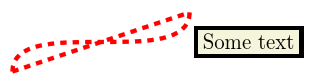
Here we can see the main parts of a TikZ picture. The picture itself is contained in a tikzpicture environment. The main components of a TikZ picture are paths, which can be drawn and/or filled (or a few other things), and nodes, which are text boxes that can be decorated.

Paths are constructed by specifying coordinates and joining them together with instructions on how the path should look between them. In the above, the first part is a straight line from (0,0) to (3,1) and the second part is a cubic Bézier curve from (3,1) back to (0,0) with the control points specified relative to their end points (this is usually the best way to specify the control points of a Bézier curve).

The number of ways to specify a coordinate in TikZ is quite possibly more than the number of particles in the known universe. The simplest is just (x,y) as x units horizontally and y vertically from an origin. It's not good to think of the origin as a fixed point on the page since the whole picture will be put in a box and positioned in the normal TeX flow (though you might well put it in a figure). Rather think of the origin as a fixed point in your diagram that everything else is relative to.

You can also use polar coordinates. This is quite useful when drawing diagrams with some rotational symmetry. To use polar coordinates, use (a:r) where a is the angle in degrees and r the distance from the origin. Note that the distance can actually be negative meaning that it goes in the opposite direction. This is surprisingly useful.

A useful modification to both of the above is to put one or more + signs in front of the coordinate. This makes the coordinate relative to the previous one. The form with only one + sign doesn't update the "base" coordinate, so in (3,4) -- ++(1,0) -- ++(0,1) then the final position is at (4,5) but in (3,4) -- +(1,0) -- ++(0,1) then the final position is at (3,5) because the ++(0,1) is taken relative to (3,4) .

Lastly, nodes can be named and then those names used as coordinates. If the node has any size, this can get quite complicated as TikZ tries to work out where on the node's boundary you meant the path to stop. There's a special zero-size node called a coordinate which acts like a bookmark for coordinates and is simply a way of labelling a particular position. This even has a special command: \coordinate (a) at (3,4); means that you can write \draw (0,0) -- (a) to draw a line from the origin to (3,4) .

Also in the above example can be seen various ways of styling TikZ stuff. There is the command \tikzset , the optional argument to the tikzpicture environment, and the optional argument to the path construction commands. Options in TikZ are specified using key-value pairs. There are even more options than ways of specifying coordinates. One thing that is very useful is the ability to gather a collection of options together into a style that can then be applied at will. This can be seen in the above example where the style my style is defined and is then applied to the \draw command.

Finally, note that every path construction command in TikZ ends with a semi-colon.

3 The Preamble

The preamble for all of these examples is the following:

\documentclass{article}
\usepackage{tikz}
\usetikzlibrary{
  knots,
  hobby,
  decorations.pathreplacing,
  shapes.geometric,
  calc
}

\tikzset{
  knot diagram/every strand/.append style={
    ultra thick,
    red
  },
  show curve controls/.style={
    postaction=decorate,
    decoration={show path construction,
      curveto code={
        \draw [blue, dashed]
        (\tikzinputsegmentfirst) -- (\tikzinputsegmentsupporta)
        node [at end, draw, solid, red, inner sep=2pt]{};
        \draw [blue, dashed]
        (\tikzinputsegmentsupportb) -- (\tikzinputsegmentlast)
        node [at start, draw, solid, red, inner sep=2pt]{}
        node [at end, fill, blue, ellipse, inner sep=2pt]{}
        ;
      }
    }
  },
  show curve endpoints/.style={
    postaction=decorate,
    decoration={show path construction,
      curveto code={
        \node [fill, blue, ellipse, inner sep=2pt] at (\tikzinputsegmentlast) {}
        ;
      }
    }
  }
}

Not every example needs all the loaded stuff, but that makes it simpler to make an example file and add all of the examples to it without worrying about packages. The stuff starting show curve ... in the \tikzset is there to help when designing knots, it isn't needed when they're finally drawn. But as the purpose of this tutorial is for you to play with the examples, diagnostic stuff is quite useful to have.

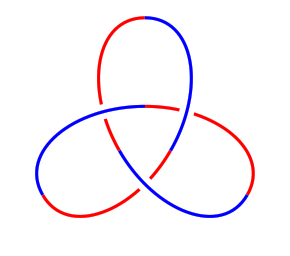
4 The Trefoil

Or rather, one of them.

\begin{tikzpicture}
\begin{knot}[
  consider self intersections=true,
%  draft mode=crossings,
  flip crossing=2,
  only when rendering/.style={
%    show curve controls
  }
  ]
\strand (0,2) .. controls +(2.2,0) and +(120:-2.2) .. (210:2) .. controls +(120:2.2) and +(60:2.2) .. (-30:2) .. controls +(60:-2.2) and +(-2.2,0) .. (0,2);
\end{knot}
\end{tikzpicture}

Let's look at this example from the inside out. The command that defines the actual path of the knot is the one beginning \strand . This is a bit like the \draw command of earlier except that it defines the path to be a strand of a knot. This particular path is defined as three Bézier curves through the points (0,2) , (210:2) , and (-30:2) with the control points defined to make the tangents at those points correct. To see the control points of the Béziers, uncomment the line show curve controls . This has the effect of drawing the tangencies.

Now let's look at the next level. The \strand command is contained in a knot environment. The environment is what does all the work with the intersections. It's possible to have more than one \strand in a knot environment, they then all get considered together.

The knot environment does a few things. Firstly, it sets up the strands so that the crossings are visible. It does this by using the double feature of TikZ whereby a path is drawn twice. The first time it draws it slightly thicker in the colour of the paper. The second time, it draws it in the colour and style requested. This makes crossings between different strands visible as each strand "wipes out" the ones underneath it.

The main work of the knot environment is to look for the intersections of the strands and provide a method whereby the crossings can be flipped if necessary.

This can be quite hard work for TeX which, after all, was originally designed as a typesetting system so the knot environment is configured by default to do the minimum work. Anything extra has to be explicitly requested.

In particular, by default the knot environment only looks for intersections between separate strands. So when we have a single strand, as here, we need to explicitly request that it look for self intersections. This is the line consider self intersections=true which is passed to the knot environment in its optional argument.

To see what it looks like without any processing, comment out the line flip crossing=2 .

Clearly, one of the crossings needs flipping and the command flip crossing=2 does this. The difficulty with using this key is clearly knowing which crossing is which. The commented out key draft mode=crossings labels the crossings so that you can see which crossing is which. Try uncommenting this to see what it does.

The cinquefoil can be obtained in a similar fashion.

\begin{tikzpicture}
\begin{knot}[
  consider self intersections=true,
%  draft mode=crossings,
  flip crossing/.list={2,4},
  only when rendering/.style={
%    show curve controls
  }
]
\strand (2,0) .. controls +(0,1.0) and +(54:1.0) .. (144:2) .. controls +(54:-1.0) and +(18:-1.0) .. (-72:2) .. controls +(18:1.0) and +(162:-1.0) .. (72:2) .. controls +(162:1.0) and +(126:1.0) .. (-144:2) .. controls +(126:-1.0) and +(0,-1.0) .. (2,0);
\end{knot}
\end{tikzpicture}

Here we have two crossings to flip. We could either list the flip crossing key once for each, or we could do what we've done here and put them together.

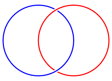
5 Links

The consider self intersections key is quite expensive: what it does is break the path into pieces and look at intersections between those pieces (the chopping up is done small enough to ensure that none of the small pieces self-intersects). With links we're looking primarily at crossings between different components so we don't need to use this splitting. Here are some link examples.

\begin{tikzpicture}
\begin{knot}[
%  draft mode=crossings,
  flip crossing=2
]
\strand (1,0) circle[radius=2cm];
\strand[blue] (-1,0) circle[radius=2cm];
\end{knot}
\end{tikzpicture}

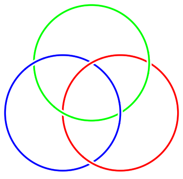
\begin{tikzpicture}
\begin{knot}[
%  draft mode=crossings,
  flip crossing/.list={3,4}
]
\strand (1,0) circle[radius=2cm];
\strand[blue] (-1,0) circle[radius=2cm];
\strand[green] (0,{sqrt(3)}) circle[radius=2cm];
\end{knot}
\end{tikzpicture}

6 Drawing Should be a Hobby

In the above examples we constructed the strands explicitly. Sometimes it is tricky to get the path looking "just right" that way. A simpler way would be to specify a set of points on the knot and draw a smooth curve through them. This is what the hobby package is designed to do. It uses an algorithm due to John Hobby to find a family of Bézier curves that pass through a given sequence of points.

(Confusingly, Hobby's paper refers to these points as knots. Another nomenclature for them is nodes. We'll just use points to avoid confusion.)

\begin{tikzpicture}[use Hobby shortcut]
\begin{knot}[
  consider self intersections=true,
%  draft mode=crossings,
  ignore endpoint intersections=false,
  flip crossing=3,
  only when rendering/.style={
%    show curve endpoints
  }
]
\strand ([closed]0,0) .. (1.5,1) .. (.5,2) .. (-.5,1) .. (.5,0) .. (0,-.5) .. (-.5,0) .. (.5,1) .. (-.5,2) .. (-1.5,1) .. (0,0);
\end{knot}
\path (0,-.7);
\end{tikzpicture}

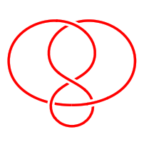
The key use Hobby shortcut enables the syntax shown in the \strand command whereby the curve is specified by listing the points separated by double dots. The [closed] in the first coordinate indicates that the curve should be a closed curve: Hobby's algorithm can work with open curves as well.

The best way to draw a knot using this method is to decide on a few key points that the strand should go through and put those in place. Then add more points to get it looking better.

This example is quite small which reveals an issue with the algorithm for finding the crossing points. Because it splits the path into segments, there are false intersections where those segments meet. By default, it ignores intersections within a certain distance of these endpoints. The key ignore endpoint intersections=false means that it takes those into consideration. This means that it might find more crossings than there should be, but that might be necessary.

When using Hobby's algorithm to draw a know, it can be difficult to see where the actual points defining the curve are. This is why the show curve endpoints was defined in the preamble. When constructing the knot, use that key to show where the endpoints are.

This is probably also a good place to note the style only when rendering . Some things about the knot strands should only have an effect when the path is actually drawn, not when the crossings are being found and not when the undercrossing is being wiped out. These go in the only when rendering style.

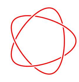
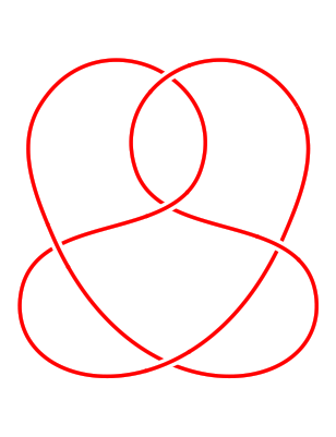
Here are some more examples using Hobby's algorithm.

\begin{tikzpicture}[use Hobby shortcut]
\begin{knot}[
  consider self intersections=true,
%  draft mode=crossings,
  ignore endpoint intersections=false,
  flip crossing/.list={6,4,2}
  ]
\strand ([closed]2,2) .. (1.8,0) .. (-2.3,-1) .. (.5,1) .. (-2,2) .. (-1.8,0) .. (2.3,-1) .. (-.5,1) .. (2,2);
\end{knot}
\end{tikzpicture}

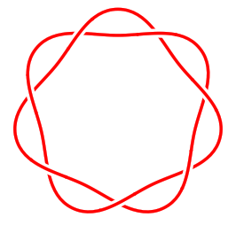
\begin{tikzpicture}[use Hobby shortcut]
\begin{knot}[
  consider self intersections=true,
%  draft mode=crossings,
  flip crossing/.list={2,4,6}
]
\strand ([closed]90:2) foreach \k in {1,...,7} { .. (90-360/7+\k*720/7:1.5) .. (90+\k*720/7:2) } (90:2);
\end{knot}
\end{tikzpicture}

7 Externalisation

If you've been copying each example into the same LaTeX document, by now it probably takes a while to compile. It's time to introduce you to externalisation.

This is a feature whereby TikZ pictures are saved to external files and then included back as images. It is quite sophisticated and can detect changes in the picture so knows when to recompile it, and there's also options for forcing recompilation.

Because of the way it works, you have to invoke your TeX command with shell escapes enabled. Different systems have slightly different ways of doing this. On Unix, you provide the commandline option -shell-escape .

There seems to be a slight issue with externalising knot diagrams in that the cropping is a bit zealous. If that seems to be the case in your pictures, a simple fix is to put the following in your preamble:

\tikzset{
  every picture/.style={
    execute at end picture={%
      \path ([shift={(-5pt,-5pt)}]current bounding box.south west)   ([shift={(5pt,5pt)}]current bounding box.north east);
    }
  }
}

I should probably figure out how to fix this bug properly.

The hobby path also has some externalisation built in whereby it is possible to save the generated data to avoid running the algorithm on every compilation. This has a nice side effect that the same path can be reused. Together with the ability to blank certain sections, this actually means that if you place the points carefully, you can draw a knot without the knots package at all.

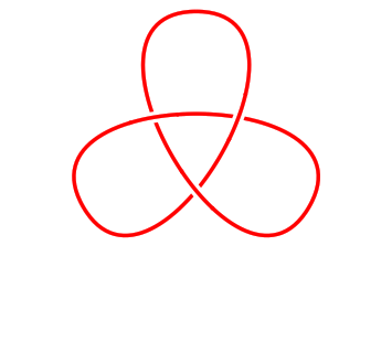
As a simple example, here's the trefoil again. It is constructed as a single path but when it is drawn then certain parts are blanked out. Then it is redrawn with the blanks and draws swapped (and in a different colour to make that easily visible).

\begin{tikzpicture}[
 use Hobby shortcut,
 every path/.style={
    line width=1mm,
    white,
    double=red,
    double distance=.5mm
 }
]
\def\nfoil{3}
\draw ([closed]0,2)
foreach \k in {1,...,\nfoil} {
 .. ([blank=soft]90+360*\k/\nfoil-180/\nfoil:-.5) .. (90+360*\k/\nfoil:2)
};
\draw[use previous Hobby path={invert soft blanks,disjoint},double=blue];
\end{tikzpicture}