1 Introduction

This is a tutorial for drawing knot, and other, diagrams using TikZ in LaTeX. It is not a tutorial for TikZ itself, though I won't assume particular familiarity with it. I will assume familiarity both with knots and with LaTeX, and a reasonable amount of ability to figure stuff out. The tutorial will be primarily example-based.

2 A Brief TikZ Primer

Having said that this isn't a tutorial for TikZ, let's start with a short description of a TikZ picture.

\tikzset{
  my style/.style={
    dashed
  }
}
\begin{tikzpicture}[line width=2pt]
\draw[my style,red] (0,0) -- (3,1) .. controls +(0,-1) and +(0,1) .. (0,0);
\node[draw,fill=Beige] at (4,.5) {Some text};
\end{tikzpicture}

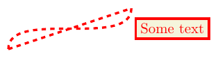
Here we can see the main parts of a TikZ picture. The picture itself is contained in a tikzpicture environment. The main components of a TikZ picture are paths, which can be drawn and/or filled (or a few other things), and nodes, which are text boxes that can be decorated.

Paths are constructed by specifying coordinates and joining them together with instructions on how the path should look between them. In the above, the first part is a straight line from (0,0) to (3,1) and the second part is a cubic Bézier curve from (3,1) back to (0,0) with the control points specified relative to their end points (this is usually the best way to specify the control points of a Bézier curve).

The number of ways to specify a coordinate in TikZ is quite possibly more than the number of particles in the known universe. The simplest is just (x,y) as x units horizontally and y vertically from an origin. It's not good to think of the origin as a fixed point on the page since the whole picture will be put in a box and positioned in the normal TeX flow (though you might well put it in a figure). Rather think of the origin as a fixed point in your diagram that everything else is relative to.

You can also use polar coordinates. This is quite useful when drawing diagrams with some rotational symmetry. To use polar coordinates, use (a:r) where a is the angle in degrees and r the distance from the origin. Note that the distance can actually be negative meaning that it goes in the opposite direction. This is surprisingly useful.

A useful modification to both of the above is to put one or more + signs in front of the coordinate. This makes the coordinate relative to the previous one. The form with only one + sign doesn't update the "base" coordinate, so in (3,4) – ++(1,0) – ++(0,1) then the final position is at (4,5) but in (3,4) – +(1,0) – ++(0,1) then the final position is at (3,5) because the ++(0,1) is taken relative to (3,4).

Lastly, nodes can be named and then those names used as coordinates. If the node has any size, this can get quite complicated as TikZ tries to work out where on the node's boundary you meant the path to stop. There's a special zero-size node called a coordinate which acts like a bookmark for coordinates and is simply a way of labelling a particular position. This even has a special command: \coordinate (a) at (3,4); means that you can write \draw (0,0) – (a) to draw a line from the origin to (3,4).

Also in the above example can be seen various ways of styling TikZ stuff. There is the command \tikzset, the optional argument to the tikzpicture environment, and the optional argument to the path construction commands. Options in TikZ are specified using key-value pairs. There are even more options than ways of specifying coordinates. One thing that is very useful is the ability to gather a collection of options together into a style that can then be applied at will. This can be seen in the above example where the style my style is defined and is then applied to the \draw command.

Finally, note that every path construction command in TikZ ends with a semi-colon.

3 The Preamble

The preamble for all of these examples is the following:

\documentclass{article}
\usepackage{tikz}
\usetikzlibrary{
  spath3,
  hobby,
  decorations.pathreplacing,
  shapes.geometric,
  calc,
  intersections
}

\tikzset{
  every path/.style={
    ultra thick,
    red,
  },
  show curve controls/.style={
    postaction=decorate,
    decoration={show path construction,
      curveto code={
        \draw [blue, dashed]
        (\tikzinputsegmentfirst) -- (\tikzinputsegmentsupporta)
        node [at end, draw, solid, red, inner sep=2pt]{};
        \draw [blue, dashed]
        (\tikzinputsegmentsupportb) -- (\tikzinputsegmentlast)
        node [at start, draw, solid, red, inner sep=2pt]{}
        node [at end, fill, blue, ellipse, inner sep=2pt]{}
        ;
      }
    }
  },
  show curve endpoints/.style={
    postaction=decorate,
    decoration={show path construction,
      curveto code={
        \node [fill, blue, ellipse, inner sep=2pt] at (\tikzinputsegmentlast) {}
        ;
      }
    }
  }
}

Not every example needs all the loaded stuff, but that makes it simpler to make an example file and add all of the examples to it without worrying about packages. The stuff starting show curve ... in the \tikzset is there to help when designing knots, it isn't needed when they're finally drawn. But as the purpose of this tutorial is for you to play with the examples, diagnostic stuff is quite useful to have.

4 The Trefoil

Or rather, one of them.

\begin{tikzpicture}
\path[spath/save=trefoil]
(0,2) .. controls +(2.2,0) and +(120:-2.2) ..
(210:2) .. controls +(120:2.2) and +(60:2.2) ..
(-30:2) .. controls +(60:-2.2) and +(-2.2,0) .. (0,2);
\tikzset{
  every trefoil component/.style={draw},
  spath/knot={trefoil}{15pt}{1,3,5},
}
\end{tikzpicture}

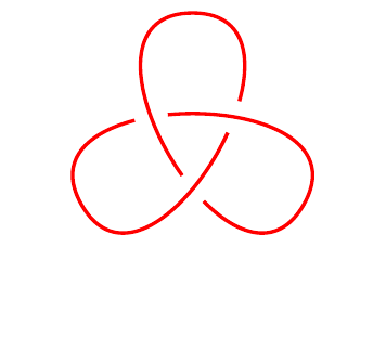
Let's look at this example. The command that defines the actual path of the knot is the one beginning \path. As this is a \path, it doesn't actually draw anything. What happens is that the path is defined and saved with the name trefoil, this is accomplished by spath/save=trefoil. This particular path is defined as three Bézier curves through the points (0,2), (210:2), and (-30:2) with the control points defined to make the tangents at those points correct.

The path so defined is a continuous, closed curve. The next part, inside the \tikzset, is what transforms it into a knot. This does several things.

First, it inserts breaks into the path at the places that it self-intersects. A break here is distinct from a gap: for a break then imagine drawing the path and lifting the pen off the paper at the break but putting it back down at the exact point it was lifted off. The purpose of this is to split the path into components, each of which runs from one crossing to the next.

Once the path is cut into components, gaps are inserted in between certain of those and the remaining breaks are removed again. In this case, the gaps are 15pt wide and they are inserted after the first, third, and fifth components. Some experimentation is needed here to figure out which components are the right ones. The next code is a useful modification that can help with that.

\begin{tikzpicture}
\path[spath/save=trefoil]
(0,2) .. controls +(2.2,0) and +(120:-2.2) ..
(210:2) .. controls +(120:2.2) and +(60:2.2) ..
(-30:2) .. controls +(60:-2.2) and +(-2.2,0) .. (0,2);
\tikzset{
  every trefoil component/.style={draw},
  spath/draft mode=true,
  spath/knot={trefoil}{15pt}{1,3,5},
  spath/get components of={trefoil}\cpts
}
\foreach[count=\k] \cpt in \cpts {
  \node[fill=white] at (spath cs:{\cpt} .5) {\k};
}
\end{tikzpicture}

As mentioned above, one of the effects of the knot key is that once the gaps are inserted then the other breaks are removed. When experimenting with where to insert the gaps, this means that the number of components changes and so it can be hard to figure out how to adjust the list of components in the knot key. The key draft mode=true stops the removal of the other breaks meaning that the components don't change (other than the insertion of the gaps). The \foreach loop then labels each component to make it easier to work with.

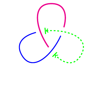
Lastly, the path is rendered. Each component is rendered as a separate path so can be separately styled. There are a variety of keys that can be used to style the components.

every spath component
spath component <number>
spath component=<number>
every <path> component
<path> component <number>
<path> component=<number>

In this example, <path> would be trefoil. The numbering of the components relates to the number after the remaining gaps were removed. So for the trefoil there are only three components.

\begin{tikzpicture}
\path[spath/save=trefoil]
(0,2) .. controls +(2.2,0) and +(120:-2.2) ..
(210:2) .. controls +(120:2.2) and +(60:2.2) ..
(-30:2) .. controls +(60:-2.2) and +(-2.2,0) .. (0,2);
\tikzset{
  every trefoil component/.style={draw},
  trefoil component 1/.style={blue},
  trefoil component 2/.style={green, dashed, |<->|},
  trefoil component 3/.style={magenta, line width=2pt},
  spath/knot={trefoil}{15pt}{1,3,5},
}
\end{tikzpicture}

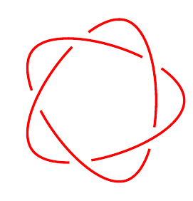
The cinquefoil can be obtained in a similar fashion.

\begin{tikzpicture}
\path[spath/save=cinquefoil]
(2,0) .. controls +(0,1.0) and +(54:1.0) ..
(144:2) .. controls +(54:-1.0) and +(18:-1.0) ..
(-72:2) .. controls +(18:1.0) and +(162:-1.0) ..
(72:2) .. controls +(162:1.0) and +(126:1.0) ..
(-144:2) .. controls +(126:-1.0) and +(0,-1.0) .. (2,0);
\tikzset{
  every cinquefoil component/.style={draw},
  spath/knot={cinquefoil}{15pt}{1,3,...,9},
}
\end{tikzpicture}

5 Links

The knot key is for a single path and combines several actions in one key. When more than one strand is involved, for example with a link, then we need to do those actions separately.

Here are some link examples.

\begin{tikzpicture}
\path[spath/save=right] (1,0) circle[radius=2cm];
\path[spath/save=left] (-1,0) circle[radius=2cm];
\tikzset{
  spath/remove empty components/.list={left,right},
  spath/split at intersections={left}{right},
  spath/insert gaps after components={left}{15pt}{1},
  spath/insert gaps after components={right}{15pt}{2},
  spath/spot weld/.list={left,right},
}
\draw[spath/use={left}];
\draw[blue,spath/use={right}];
\end{tikzpicture}

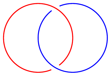
In this example there are several important keys. The first key, remove empty components, is useful for simplifying matters a little. Some path constructions, such as the circle, leave extra moves in them. These can make it tricky to keep track of which component is which, so getting rid of them can be useful.

The middle key inserts breaks where the two paths intersect, and then the next two keys insert the gaps. Finally, the last two keys remove the breaks which didn't have the gaps inserted.

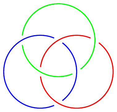
\begin{tikzpicture}
\path[spath/save=right] (1,0) circle[radius=2cm];
\path[spath/save=left] (-1,0) circle[radius=2cm];
\path[spath/save=upper] (0,{sqrt(3)}) circle[radius=2cm];
\tikzset{
  spath/remove empty components/.list={right,left,upper},
  spath/split at intersections={left}{right},
  spath/split at intersections={right}{upper},
  spath/split at intersections={upper}{left},
  spath/insert gaps after components={left}{15pt}{2,4},
  spath/insert gaps after components={right}{15pt}{1,3},
  spath/insert gaps after components={upper}{15pt}{1,3},
  spath/spot weld/.list={right,left,upper},
}
\draw[blue, spath/use={left}];
\draw[red, spath/use={right}];
\draw[green, spath/use={upper}];
\end{tikzpicture}

6 Drawing Should be a Hobby

In the above examples we constructed the strands explicitly. Sometimes it is tricky to get the path looking "just right" that way. A simpler way would be to specify a set of points on the knot and draw a smooth curve through them. This is what the hobby package is designed to do. It uses an algorithm due to John Hobby to find a family of Bézier curves that pass through a given sequence of points.

(Confusingly, Hobby's paper refers to these points as knots. Another nomenclature for them is nodes. We'll just use points to avoid confusion.)

\begin{tikzpicture}[use Hobby shortcut]
\path[spath/save=figure8]
([closed]0,0) .. (1.5,1) .. (.5,2) ..
(-.5,1) .. (.5,0) .. (0,-.5) .. (-.5,0) ..
(.5,1) .. (-.5,2) .. (-1.5,1) .. (0,0);
\tikzset{
  every spath component/.style={draw},
  spath/knot={figure8}{15pt}{1,3,...,7}
}
\path (0,-.7);
\end{tikzpicture}

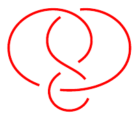
The key use Hobby shortcut enables the syntax shown in the \strand command whereby the curve is specified by listing the points separated by double dots. The [closed] in the first coordinate indicates that the curve should be a closed curve: Hobby's algorithm can work with open curves as well.

The best way to draw a knot using this method is to decide on a few key points that the strand should go through and put those in place. Then add more points to get it looking better.

When using Hobby's algorithm to draw a knot, it can be difficult to see where the actual points defining the curve are. This is why the show curve endpoints was defined in the preamble. When constructing the knot, use that key to show where the endpoints are.

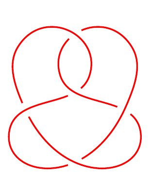
Here are some more examples using Hobby's algorithm.

\begin{tikzpicture}[use Hobby shortcut]
\path[spath/save=5-2]
([closed]2,2) .. (1.8,0) .. (-2.3,-1) .. (.5,1) ..
(-2,2) .. (-1.8,0) .. (2.3,-1) .. (-.5,1) .. (2,2);
\tikzset{
  every spath component/.style={draw},
  spath/knot={5-2}{15pt}{1,3,...,9}
}
\end{tikzpicture}

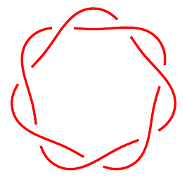
\begin{tikzpicture}[use Hobby shortcut]
\path[spath/save=7-1]
([closed]90:2) foreach \k in {1,...,7} {
  .. (90-360/7+\k*720/7:1.5) .. (90+\k*720/7:2)
} (90:2);
\tikzset{
  every spath component/.style={draw},
  spath/knot={7-1}{15pt}{1,3,...,15}
}
\end{tikzpicture}

7 Externalisation

If you've been copying each example into the same LaTeX document, by now it probably takes a while to compile. It's time to introduce you to externalisation.

This is a feature whereby TikZ pictures are saved to external files and then included back as images. It is quite sophisticated and can detect changes in the picture so knows when to recompile it, and there's also options for forcing recompilation.

Because of the way it works, you have to invoke your TeX command with shell escapes enabled. Different systems have slightly different ways of doing this. On Unix, you provide the commandline option -shell-escape.