Monotillic Musings
2025-03-22

Contents
1 Introduction
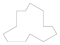
The recent (at time of writing) announcement of an aperiodical tile, as in Figure 1, caught my attention for more than just the "Oh, this is interesting" reason.
I have two pieces of code that were originally developed for exploring Penrose tiles and so my first reaction was to include the new tile in those. That meant a fair bit of code refactoring1, but also a close examination of the new tile from a different perspective than if I'd just been exploring it as a tile.
1Mainly because the original code is relatively old and I've learnt a bit about programming since I originally wrote them.
The two programs are a TikZ library for drawing tilings and the other is a program I wrote using the iPad app Codea. Both originally were written specifically for Penrose tiles, but have been extended in the years since they were first devised.
Key features of the TikZ library are:
-
There is a mechanism for placing tiles alongside previously placed tiles.
-
There is an implementation of the substitution system for Penrose tiles.
-
The edges of the tiles can be deformed (consistently).
Key features of the Codea program are:
-
It is interactive, so tiles can be drag-and-dropped into a design (with a snap against existing tiles).
-
It can check whether a tile is in a valid position, not just against existing tiles but also whether the tile will lead to an impossible position (with a finite lookahead).
-
It can fill in forced tiles.
-
It has a recursive mode that will fill in forced tiles, then place a random (valid) tile, and iterate that to fill the screen.
-
It can apply the substitution rules.
-
It can export a design suitable for importing with the TikZ library.
The validity testing and the generation mode both rely on the same underlying idea which is that when a tile is placed (either by hand or automatically) then the program will test its exposed edges to see if it is possible to place a tile next to each one that doesn't overlap the existing pattern2. This means that the program needs to know which edges can go alongside each other.
2This is the first level of checking, it can be made deeper. The normal Penrose tiles only needed one level of checking, but the pentagonal system needs two.
So my initial focus with the new tiles was to look carefully at the matching rules. I also wanted to include at least some of the clusters (super, meta, sub) in my code to make the programs as broadly useful as I could. The remark about the subclusters being awkward (starting on p16 of the preprint) intrigued me as well and this led to me looking at the subclusters more closely.
In this closer examination of the subclusters my attention was drawn to the and tiles in particular. These are especially interesting as they seem designed to allow alternative edge matches to those permitted "by default". That is, if we view the labelling of the edges in the Figure at top of p18 of the original article as the default matching rules for the and subclusters then the and provide exceptions to these rules.
Perhaps the mathematical habits of a lifetime came into play here and prompted me to focus for a bit on those exceptions. Indeed, removing the and tiles and looking just at the and provides interesting structures. These have been highlighted by others – including in the original paper – in regard to the super and meta clusters; I think that including the subclusters in this analysis is particularly illuminating.
This focus feeds in nicely to considering the substitution rules. With both the TikZ and Codea programs then I've found the substitution mechanism to be both useful and interesting. So it is a little disappointing that there isn't a direct substitution system for the polykite tiles themselves. Implementing them for the super clusters is straightforward, though, and for the TikZ library then I've adapted it to use the combinatorial substitution rules to generate polykite tilings. My current implementation for the Codea program uses the positional information more integrally so is a bit trickier to adapt to the neighbour information. So at the moment, the Codea program only implements the substitution system for the super clusters.
2 Matching Rules
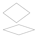
A key feature of the standard sets of Penrose tiles is that they have matching rules. These can be enforced by deforming the edges but it is more common to decorate the tiles with arcs that have to align, as in Figure 2.
The new tile, which I'll call an aperiodical hat, doesn't need matching rules. It is made up of edges of two lengths3 and there are no a priori restrictions on which edge can match with which. So my first implementations, both for the TikZ library and the Codea program, allowed any edge of a given length to match or align with any edge of the same length.
3There is one extra long edge which is actually best viewed as two short edges.
The problem with this is that there are several of each, and this causes issues for both programs. When using the TikZ library I found myself continually counting and losing count of the edges and having to remember where the starting point was. The Codea program uses the matching rules to test whether a tile is valid by trying to place tiles next to it and if there are lots of ways a two tiles can be placed next to each other then this process is very slow.
In fact, it is even worse than just a linear increase. That there are many possible edge matches, but not all will be eventually valid, means that when checking a tile is valid then it is necessary to try placing not just one extra tile next to it but maybe two or more. If I can figure out some edge combinations that could never occur in a valid pattern then I can rule them out as potential matches from the outset and so make it easier to create patterns in both programs.
So for both programs I wanted to have a better understanding of the possible edge matchings. Because the subclusters (at least, the and tiles) are themselves hat tiles, I thought to examine them a little more closely to see if they could shed light on how the hat tile itself worked.
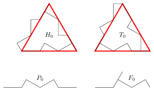
The diagram at the top of p18 and partially reproduced in Figure 3 is particularly intriguing. It is clear from that diagram that the individual edges of the hat tile are best thought of not separately but grouped. Also, the whiskers – and the comparison with the meta and super cluster tiles – show that these tiles should really be thought of as deformed equilateral triangles. So in the TikZ library, the subcluster tiles (that is, the and tiles) are actually equilateral triangles with a specific edge deformation already applied.
This means that the subclusters are actually the most straightforward way to use the TikZ library at the moment, as there are only three edges for each of the main tiles, as in Example 4.
\begin{tikzpicture}[
  every subcluster H/.style={draw, thick},
  every subcluster T/.style={draw, thick},
  every subcluster F/.style={draw=red, ultra thick}
]
\pic[subcluster H, name=A];
\pic[subcluster F, name=B, align with=A along b1];
\pic[subcluster F, name=C, align with=B along f];
\pic[subcluster F, name=D, align with=C along f];
\pic[subcluster H, name=E, align with=C along b using 1];
\pic[subcluster H, name=F, align with=D along b using 1];
\end{tikzpicture}
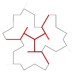
Figure 4: Example of positioning subcluster tiles
This approach doesn't work for my Codea program as that hasn't been designed to allow for tile deformation, so I need to work with the original tiles4. However, the subcluster matching rules can be used to refine those for the hat tiles.
4For implementation reasons, I was already working with the original tile and its reflection.
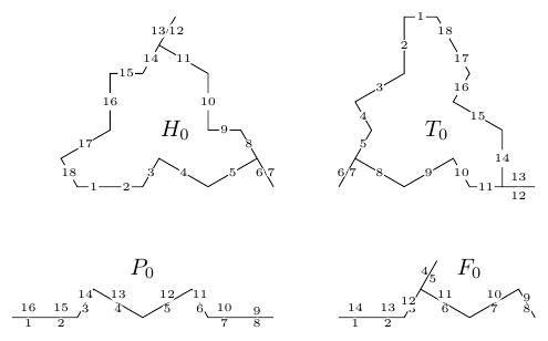
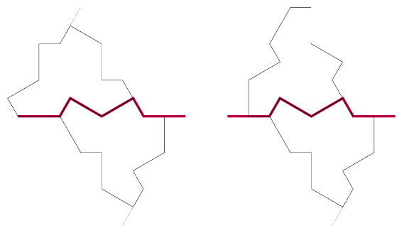
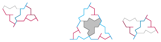
The first step in this analysis is to label every segment of the subcluster tile paths, including the whiskers and also regarding the longest segments as two short segments. This is shown in Figure 5.
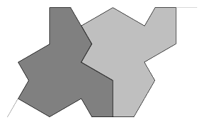
Let's start with the subcluster. The matching rules for the subclusters determine most of the matching rules for the individual edges directly, as in Figure 6.
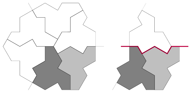
Sides to of match against to or to of . Sides to match against to of as do to . This leaves just sides and . To figure out what happens with these, consider Figure 7.
The top edge of the tile can be matched by either a , , or . The and both then force tiles that mean the original is completely surrounded. The leads to an overlap meaning that it actually doesn't fit. So the possible patterns are as in Figure 8, which means that sides and of match against each other and against and (respectively) of . We'll see later that the left-hand side of Figure 8 is actually not possible so we can exclude the match between sides and of .
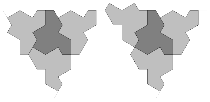
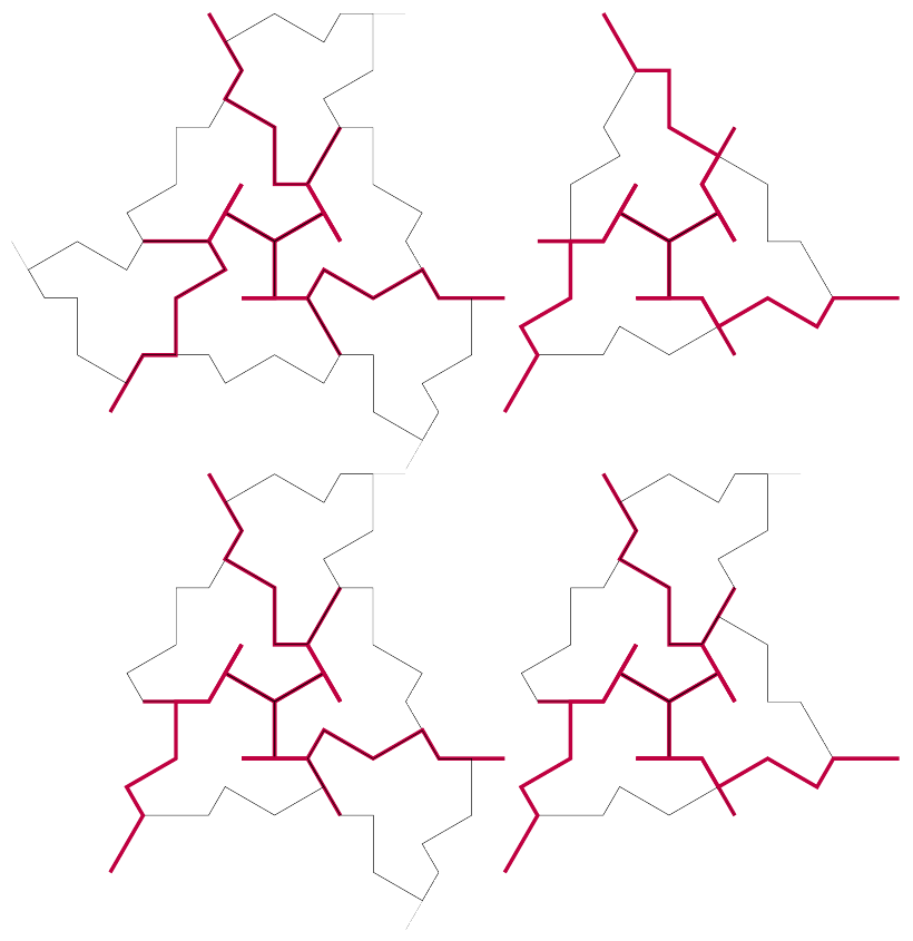
The tile obviously has a lot more possibilities. Obviously, all the matches to edges on are already accounted for so the focus is on matching with itself. Figure 6 shows that edges and match but other than that, the self-matches of must involve the or tiles. The two edges on an subcluster tile give two ways that the directly attaches to s, as in Figure 9. For the subcluster tile then it makes sense to put three together as that is the only way that the edges can match, then there are four ways of directly attaching these to s, as in Figure 10. After attaching each , the that attaches to the inner edge of each is forced and if the edge of the is free then that forces an .
The tiles provide matches between , , and with each of , , and , , .
The tiles provides matches as follows:
-
, and , .
-
, , and , , .
-
, , and , , .
-
, and , .
Lastly, we need to look at how the and tiles can be combined. These will adjoin along their edges. At first sight there are several ways that these can combine but in fact it can't be that two tiles adjoin.
The tiles can align in multiple ways, both with themselves and with s. The focus is on how the edges match, since the edges on an can only align with another edge on another – so the s always come in threes. The s on an can either match with any other edge except that the inner cannot align with itself.
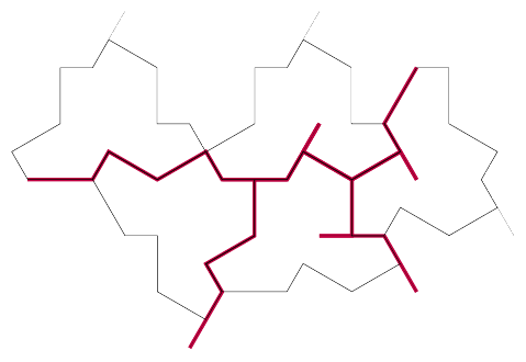
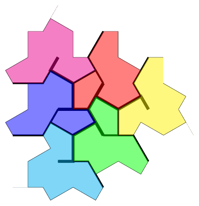
A few of the possibilities are shown in Figures 11, 12, and 13. In the last of these, I've used a more colourful design partly because it looks nice and partly because the way that the tiles intersect their neighbouring s means that it can be tricky to see which part of an belongs to which tile.
Most of these yield combinations already encountered, but Figure 11 produces a match between the pair and with and while Figure 12 pairs and with each other. Also, the right-hand side of the lower right diagram in Figure 10 shows that sides and match.
I claim that this is all the matches that can happen. To verify that, I can create a list that I know must contain all possible matches but which might have some that cannot actually occur and then look at the difference between the two lists. To make that list, I consider how edges align under the subcluster matching rules including the whisker edges on the and tiles. Then I trace how edges match up.
For example, edge of matches with edge of . Edge is back-to-back with edge (of ), so anything that edge of matches with is a potential match for edge of . By tracking these potential matches, I can make a list of all the potential matches. I have a Python program to create this list.
The excess matches that this throws up are:
-
edge has extra matches against edges , , and edge .
-
edge has extra matches against edges and .
-
edges and have extra matches against each other.
We've already examined edge of and seen that it can only match against edge . The other potential matches all directly lead to overlaps and so are clearly invalid. Therefore, we have found the entire set.
Lastly on this, my iPad program can use this information to generate a tiling by successively adding tiles to an existing pattern. To do this, it obviously uses the matching rules to try to place a tile against an already placed one. But just because a tile matches against the existing pattern doesn't make it a valid tiling because it might lead to an invalid patch further down the road. As an attempt to avoid this, my program uses the following scheme:
-
Say that a positioned tile is –invalid if it overlaps an existing tile.
-
Say that a positioned tile is –invalid if it has an exposed edge with the property that every possible matching tile positioned along that edge is –invalid.
The base level of invalidity is the most obvious one: the tile can't be physically placed because existing tiles block it. The next level works like this. The tile itself works, in that it is validly placed without overlapping existing tiles and it matches wherever it has an edge in common with the existing pattern, but when we try to place tiles around it then we can't. There is at least one edge where whenever we try to place a tile then it overlaps the existing pattern. Note that we don't look for a simultaneous surrounding of the tile, just each edge in turn.
So the program has a checking depth which means that when it tries to place a tile then it checks its validity to that depth. With kite-and-dart and rhombii Penrose tiles then I found it only necessary to check if a tile was –invalid. With the pentagonal Penrose tiles then I had to go to level .
I've not yet determined how deep the aperiodical hats have to go. I sometimes get a valid pattern with checking depth , but not always.
3 Charge
Maybe it's because I occasionally talk to particle physicists that the subcluster diagrams put me in mind of a couple of things from that field. The and "tiles" look very much like particle tracks, and the choice of for the edge matches puts me in mind of charge conservation.
I'll start with the second of these. Looking at the charges on their edges, it is clear that each and tile has net charge , the tiles are neutral, and each tile has net change . We can use this to look at how the subcluster tiles are put together.
The charge is also geometric in that the and tiles are essentially equilateral triangles with deformed edges. The deformations, though, are not balanced in that the deformed path cuts away part of the tile and so each and has less area than its underlying equilateral triangle. However, they can only be placed as if they were equilateral triangles. So eventually, the deficit (or charge) builds up until it needs addressing.
The other aspect that we need to bring in is the structure of the and tiles. An tile has to form part of a triumvirate and those three tiles produce six edges which must match tiles. The underlying shape of a tile is a straight line and at its ends it must match either another or an . So from an triumvirate then six lines emanate travelling in the six hexagonal directions (though not co-central) and these are continued along s until they encounter another . This means that the s and s carve up the plane into triangular areas which are filled with s and s.
Since each matched edge is neutral, the net charge inside a region must be visible on its boundary. An equilateral triangular region with equilateral triangles on its edge has triangles in its interior, so as each of those triangles is an or it has a net charge of . Each edge can transmit only one unit of charge, so the maximum charge across the boundary of such a triangular region is . Therefore, the maximum size of a triangular region is when which means that .
However, this largest size is not possible. The reason being that along one of its edges there would have to be two s both pointing inwards meaning that they are pointing outwards of the next area and this can't happen. This can be seen at the bottom of Figure 14 where there is an unfillable region.
So the possible regions have size or , as in Figure 15.
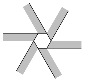
Now the triumvirates have to contribute charge. Geometrically, this means that they have to somehow compensate for the area deficit between viewing the tiles as equilateral triangles and the actual deformed tiles. I think of the way that they do this as analogous to techniques from origami tessellation. When folding a tessellation pattern then there can come a point where one has "too much" paper at a location whereupon a twist is done to use up the excess paper. In Figure 16 then the grey lines are where the paper overlays itself via a fold with the black edges as the visible edge. Six such folds meet –roughly – at a point where a hexagon is formed to flatten the connection.
In this way, the triumvirates can introduce "charge" – equivalently, compensate for the area deficit – by offsetting the regions against each other. The s along the sides of the regions then perpetuate this offset.
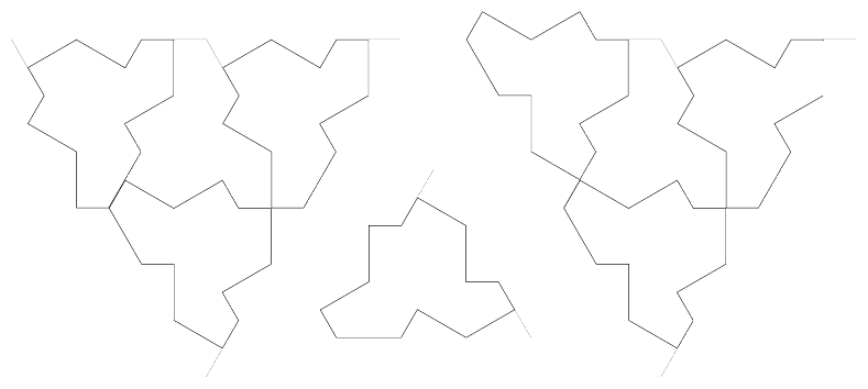
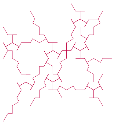
Focussing on the regions like this also brings in the other "particle physics" aspect: the jagged lines looking like particle tracks. By drawing just the outlines – so the and tiles – and not the and s then it will look like particles splitting and recombining at the s and travelling along the s. Adding a little animation to this would be fun!
4 Substitution Rules
I use the substitution rules for the Penrose tilings with both my iPad and TikZ code as a way to generate a tiling of a large area. Unfortunately, the substitution rules for the polykite tilings are a little more complicated as the true substitution system only works for the super clusters. However, the combinatorial data for a super cluster tiling can be used for a subcluster one so it is theoretically possible to generate a super cluster tiling using the substitution rules and then use the adjacency information to generate a subcluster tiling.
There's a very nice posting about this, and similar topics, which points out an issue with this in that the two tilings will cover different regions. However, for my use cases then this isn't a big factor – with the TikZ library, for example, it is never going to be the most computationally efficient way to draw a large patch – if one wanted to do that then a better strategy would be to generate a tiling by some other program which is then imported into TikZ. The more likely scenario for using the substitution rules is just going to be to draw a relatively small patch directly. Similarly, my iPad program isn't designed to produce extremely high resolution diagrams but just be a way to explore the tilings at "human" scale. So in both cases a bit of trial and error to get the right region will not, I think, be a huge drawback.
A more significant snag is that my original implementation of the substitution systems for Penrose tilings – in both the iPad and TikZ code – worked purely on positional information. So it was simplest to start with the super cluster substitution systems.
4.1 Super Clusters
Both my iPad and TikZ library have implementations of the super clusters so although my feeling is that they were introduced as a means to an end, it is nevertheless perfectly possibly to implement the substitution system directly for the super clusters using my existing framework.
In the TikZ library, the substitution rules work as follows. Starting with a seed string of characters, it applies replacement rules to each of those characters in turn. This is repeated until the required depth is obtained, at which point it switches from rules to actions. These interpret the symbols to, eventually, draw the tiles at certain locations and in certain orientations.
The dictionary of symbols that I use for the super clusters is:
-
H,T,P,Frepresent the tiles themselves. In the replacement stage these are successively replaced by longer strings and in the action stage these represent the actual tiles. -
sdenotes scaling by . In the replacement stage then the transformation symbols are not themselves replaced (but are left in the string). -
x{..},y{..}. These all represent a movement by a certain step horizontally or vertically (relative to the current coordinate system). The units are set so that these move on a hexagonal grid. -
r{..}. This rotates by its argument. -
[and]. These introduce scoping so that transformations only apply within their scope.
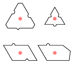
The replacement rules are so that each tile is replaced by one or more tiles at a scale of with certain positions and rotations. The positions and rotations depend to some extent on the orientations of the tiles. The original paper does not settle on a particular orientation for the clusters but rather draws them in different orientations at different places in the paper, as appropriate for the work of the given section. For the replacement rules, I've used the orientations as in Figure 18. Also important is to identify the "origin" of each tile. For the , , and tiles I've set the origin to be its centre. For the tile, imagine overlaying it with a tile in the obvious way and fix its centre at the same as for the tile.
With these orientations, the replacements are as follows.
-
a super cluster is replaced by a single at the same location and rotation.
-
an super cluster is replaced by a tile, and three of each of , , and with the following positions and rotations.
-
The tile is at rotated by .
-
The tiles are at , , and with the first two not rotated and the last with a rotation of .
-
The tiles are at , , and with respective rotations , , and .
-
The tiles are at , , and with respective rotations , , and .
-
-
A tile is replaced by another tile, two tiles, and two tiles with the following positions and rotations.
-
The tile is at rotated by .
-
The tiles are at and with respective rotations and .
-
The tiles are at and with respective rotations and .
-
-
An tile is replaced by a tile, two tiles, and three tiles with the following positions and rotations.
-
The tile is at rotated by .
-
The tiles are at and with respective rotations and .
-
The tiles are at , , and with respective rotations , , and .
-
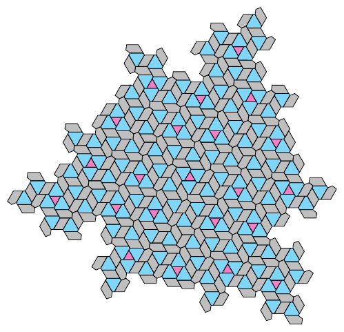
Figure 19 shows a result of this substitution system.
4.2 The and Substitution Rules
On page 18 of the preprint, there is an alternative substitution system not based on the clusters but on two groupings of tiles, one with tiles and one with . I initially thought this might be a positional substitution system so spent a little while thinking about implementing it. I no longer think that it is positional, based on trying to get the second level of substitutions to line up. It may be that I am not interpreting it correctly, but I've decided to leave it for the time being.
However, while investigating it then I did discover something interesting. I wanted to work out the ideal area scale factor, so looked at the long term behaviour of the system. Each tile is replaced by a single and five s, while each by a single and six s. So if there are lots of and lots of prior to a substitution then there will be lots of and lots of afterwards. In the long run, this should stabilise so that the ratios of s to s is constant.
One way to investigate this is to set it up as a matrix equation:
To find out what happens in the long run we look at the eigenvectors and eigenvalues of the transition matrix. This has characteristic polynomial:
The solutions of this are:
The dominating eigenvalue is and it has eigenvector
So in the long run, the ratios of s to s converges to . In the limit, a single substitution multiplies the numbers of both s and s by , so this is the area scale factor.
The numbers and are ones that I've encountered before. This introduces a new angle on those Golden Numbers. The Golden Ratio itself, , can be found in the ratios of the eventual fate of the golden triangle and golden gnommon under their substitution rules and these are linked to Penrose tiles. So maybe each of the Golden Numbers can be associated with a tiling by a pair of tiles, say and , so that in the substitution then each of and are replaced by a single and some number of s where the numbers of s differ by . In the notation of the Golden Numbers post, the ratio of s to s would then be some .
4.3 Neighbourly Substitutions
For the other families of tiles, if I want to use the substitution system then I need to figure out a way to retain the neighbour information.
When placing a tile, I need to know:
-
The type of tile (, , , or );
-
Its neighbour to position it against;
-
The edge of the neighbour to use;
-
The edge of the new tile to use.
The TikZ library accesses tiles via labels, so the second item on that list can be the label. It will be useful for the replacement system to also note the type of the neighbour tile, and its own label. Therefore, a tile is stored as a token list consisting of the type, label, and edge of both the new tile and the neighbouring tile. An example of such is:
{HTa{A1}} {01} {00}
This represents a tile of type with label which is placed next to an existing tile of type with label . The edge of the tile is placed next to the edge of the tile. Note that in the encoding system, the edges are labelled for and for , and where a tile has multiple edges of the same type they are , etc. The braces are for implementation reasons so that the code "sees" this in a particular way.
Now when this tile is replaced, then the tile becomes new tiles (a , and three each of , , and ) while the tile becomes an tile. The new tile (replacing the ) is placed first and then the tiles from the are placed afterwards, starting with one of the tiles that is adjacent to the tile. The order of placing these new tiles will depend on which edge is used to place the original tile, meaning that there needs to (potentially) be replacement rules for every possible pairing of two tiles next to each other.
The current implementation is actually slightly shorter because unless the starting conditions are chosen specifically then every tile can be placed using an or type of edge, so only replacement rules for these need to be specified. In addition, there are a few shortcuts on creating the rules that I was able to exploit which made it relatively straightforward to code.
I even got to the point where my first guess for the rules was the right one, which was helped considerably by spotting that under the replacement rules then edges and edges swap. So that if, as above, an tile was placed next to a tile along an –type edge then in the replacement a tile (of the ) will end up next to the (of the ) along a –type edge.
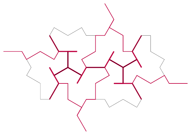
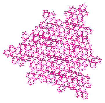
With this, it is now possible to create diagrams such as Figure 20 in only a few lines of code.
4.4 Subclusters
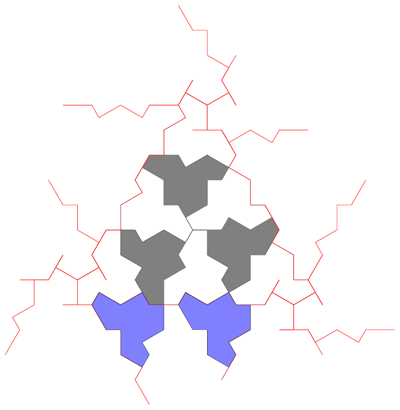
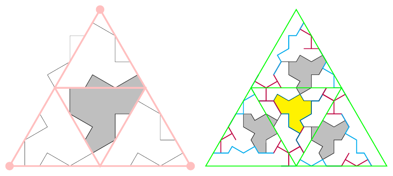
The subclusters have the same structure as the other clusters so it is interesting to see what happens to those with the substitution rules.
Figure 21 shows the replacements for the individual tiles, except for which is simply replaced by an . Figure 22 shows a possible substitution for a set of tiles surrounding a . What is interesting about this substitution is that it looks as though the scale factor is and that the extra space needed for the tiles introduced by the and substitutions comes about by folding space, reminiscent again of tessellation origami.
5 Conclusion … for now
I'm quite pleased with what I've been able to implement in both the TikZ library and the Codea program. Getting the combinatorial substitution rules into the Codea program would require a fair amount of code refactoring that I'll shelve for the time being, but having it for the TikZ library feels quite significant.
There's plenty to continue investigating, and the relationship between tiling sets and Golden Numbers is intriguing.
For now, though, this seems like a reasonable place to pause on the development and maybe write up some documentation.